The practical application of psf models has already been alluded to (see Sections 3.3 and 4.4). The advantage of psf models over simple psf access is purely one of processing time. Injudicious selection of parameters can result in either poor representation of the spatial variation of the psf or even more processing time being expended than with simple access.
The model psfs should be used in conjunction with applications which have the facility to support spatially variable psfs,
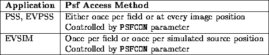
When using PSS or EVPSS it is almost always worthwhile using a model to represent variable psfs, as access is so intensive. The psf access time for EVSIM will only dominate for large numbers of sources, so the model option is only worthwhile in that situation. All other applications using the psf system cannot benefit from the use of model options.
The two model options work on a similar principle. The model specifications define a grid of a finite number of psfs. Each access to the psf system by an application at a given image position then extracts the psf from the grid bin containing that position. Psfs are are only calculated as they are needed, so not even the number of psfs in the grid need be calculated. The first argument of each model specification is an instrument psf name from the first display group.
The POLAR option sets up a grid whose bin boundaries form lines
of constant radius and/or azimuth in polar coordinates. The most simple
form of a polar psf grid defines only regularly spaced radial bins. For
example,
POLAR(XRT_PSPC,0.04)defines a grid of the ROSAT PSPC psf where the radial bin boundaries are 0.04 degrees apart (floating point values in model specifications are always in image axis units). The psf system automatically finds the number of radial bins from the image centre to the extreme corner. The first complication is to allow non-regular radial bins,
POLAR(XRT_PSPC,0.05:0.1:0.2:0.5)This example defines bin boundaries placed at to 4 specified radii (see Ref 5,`` User Interface,Lists and ranges" for a description of bin boundary syntax). The psf system supplies additional boundaries of zero and infinity. The third optional argument for a polar model is an integer, the number of azimuthal bins. By default this is one, but any number can be specified. The specification,
POLAR(XRT_PSPC,0.05:0.1:0.2:0.5,4)defines 4 azimuthal bins. The boundary of the first starts at the algebraic angle zero degrees, proceeding round the image centre at intervals of
 degrees. A special case is the central
radial bin, which always has only one azimuthal bin. This
prevents subdivision of the image centre into very small grid bins
ensuring continuous psf data across this area (where there is greater
likelihood of there being a source).
degrees. A special case is the central
radial bin, which always has only one azimuthal bin. This
prevents subdivision of the image centre into very small grid bins
ensuring continuous psf data across this area (where there is greater
likelihood of there being a source).
The RECT option sets up a grid whose bin boundaries form lines
in constant image ordinate or abscissa. Again the third argument is optional,
but in the RECT option the default is to assume in the same
specification as defined in the second argument. Again there is a
regular and an irregular form,
RECT(PWFC,5)defines a regular grid of spacing 5 arcminutes in both axes, whereas
RECT(PWFC,-60:-40:-20:-10:0:10:20:40:60)defines an irregularly spaced grid. The third argument, if specified, has the same syntax as the second.
The precise grid to define depends on the instrument, some guidance can be found in Ref 5,`` User Interface,Psf System". Once the psf model has been specified, the MASK and AUX prompts may appear to get additional information for the instrumental psf.