IDL_HS Version 4: User's Guide

James Tappin

1 Introduction
- 1.1 Capabilities
- 1.2 What has not been re-implemented
2 The internal structure of IDL_HS Version 4
3 The Shell Command
4 IDL_HS User Interface
5 Top level
6 Rate datasets
- 6.1 Streams
- 6.2 Postprocessing
7 PAD datasets
- 7.1 Streams
- 7.2 Postprocessing
8 Spect Datasets
9 Dynamic Spectrum Datasets
- 9.1 Streams
- 9.2 Postprocessing
10 Matrix Datasets
- 10.1 Postprocessing
11 Activity Plots
- 11.1 Postprocessing
12 Settings common to several dataset classes
13 The data editor
14 Other parts
- 14.1 Plot settings
- 14.2 Examine File
15 General Points
- 15.1 Modal Menus
- 15.2 Backgrounds
A. UDS data and its specification.
B. Default settings and customisation
- B..1 rc_maker
- B..2 Defined resources
About this document ...

1 Introduction

The aim of this guide is to provide an introduction to the operation of version 4 of the HISCALE/EPAM display environment.

Initial development was on Solaris systems, the current development platform is Linux. All development has been done with IDL version 5.2, 5.4 and 5.5. The system should work on most Unix flavours supported by IDL. VMS support will need someone with DCL expertise to create a script to run the system. Support for Windows or Mac would need major work.

This document refers to the fifth full release series (Versions 4.6.x: Ida).

1.1 Capabilities

Time-series plots (rate datasets):
- HISCALE and EPAM rates data.
- ULEIS matrix rates data.
- HISCALE and EPAM track data.
- HISCALE and EPAM MFSA 32-channel data¹.
- Merged magnetic field data.
- UDS data. This includes any data stored in a reasonable ASCII format, so that a spec file can be written for the file.
The calculation of ratios and/or spectral indices between different channels is supported, although in a different (and I hope better) way from version 3.
Channels of different types may be combined in the same dataset (so for example you could plot an EPAM composition channel, a ULEIS channel and the ACE magnetic field magnitude on the same page).
Pitch-angle plots for HISCALE, EPAM and ULEIS rates data (pad datasets).
The layout engine is much improved compared with version 3.
Spectrum plots (spect datasets):
- HISCALE and EPAM rates data.
- ULEIS matrix rates data.
- HISCALE and EPAM track data.
- HISCALE and EPAM MFSA 32-channel data.
As with rates datasets, different types of data can be mixed in a single dataset.
PHA Matrix plots for HISCALE and EPAM data (matrix datasets).
The main change from version 3 is that it is now possible to sum (or average) matrices. It is also possible to select non-square subfields to display.
X-ray flare activity plots (xflare datasets).
It is now possible to select Bartels or Carrington rotations and longitude. Histograms of the longitude and/or time distribution can be added to the plots.
Dynamic spectrum datasets, similar to those in the old fortran software; but now including Track and Uleis data.
An HSIO file browser.
A system of resource files to allow customization both by site and by user. It is possible to support multiple platforms from a single software tree.
GUI to control it.
A CLI / Scripting interface.
A data editor to allow the removal of telemetry errors and calibration spikes.

1.2 What has not been re-implemented

CDF data. Because it isn't widely or regularly distributed to the team and it contains less channels and at a lower time resolution than the UDS data.
MOVIE. Because it isn't very useful, PAD plots provide a much more quantitative measure of anisotropy. Also the way that it works was restricted to 8-bit display depths.

2 The internal structure of IDL_HS Version 4

The conceptual structure of version 4 is very different from that of its predecessors, so a brief description will probably help you to understand how to do what you want to do. For what it's worth, most of the code is implemented in object-oriented IDL, but unless you are developing software, that need not concern you. However the organization should.

In the earlier versions, there were several display programs which shared certain properties (time range etc.) while each had its own data storage arrays (apart from plot_rates and movie which shared many arrays). The data were associated with a program and as a result looking at a new set of data with a particular program or changing a shared property destroyed the data previously read.

In version 4 the new pointer and object capabilities of IDL version 5 have been used to break this limitation. This is done by introducing the concept of a dataset, which has its own properties and is associated with a form of display (time-series, spectrum, PAD distributions etc.) but which is independent of all other datasets. Each dataset is then subdivided into streams which correspond to a single channel for the old plot_rates and plot_pad programs, and to a head or species in plot_spect or plot_comp. In the case of pad and spect datasets, the streams are grouped into panels. The major advantage of this scheme is that it allows two major new freedoms:

It is now possible to combine data of different classes or from different instruments on a single plot. This was the main reason for the development of version 4.
It is possible to have simultaneously present datasets of the same type but with different data (including different time ranges, averaging etc.).

To provide consistency and convenience, IDF information and plot settings are shared between all datasets. However, information in a particular stream that is derived from the IDF will not be updated when the IDF is changed.

A dataset contains all the information needed to create a plot. It also has internal flags to ensure that its status is correctly known to the software. The easiest way to think of a dataset is as equivalent to the old routines such as PLOT_RATES, except that you can have multiple datasets of any one type. When it is created, a dataset can inherit the "global" properties of an existing dataset², but thereafter they are entirely independent entities.

In earlier versions of the software, each program was provided with a list of channels (whether these be a LAN channel as in PLOT_RATES or a head as in PLOT_SPECT). In version 4, the channel is replaced by the stream. A stream contains the data for a channel and also the IDF information relevant to that channel (e.g. the energy range and background levels). In addition if a particular channel has different sectoring or scaling options from the defaults for the dataset, then the stream also stores these.

When data are read, the dataset controls the reading and then passes the relevant bits to the various streams, this way we can separate the data up without having to make multiple passes through each data file.

Whereas previous versions had a single data directory which served for all programs; version 4 has a number of data paths. These paths are associated with the IDF settings and are real search paths. Thus it is possible to have separate search paths for HISCALE and EPAM, and for rates data and for track/pha data, and in addition these may consist of several directories (e.g. your ULA and CUAF directories).

The plotting setup is very similar to earlier versions except that the spool command is now defined in the setup menu and also there are separate spool commands for printable and encapsulated files.

Internally, all times are now stored as julian-day numbers. Energies are stored in MeV, but for any dataset³, display in MeV-based units or keV-based units is selectable.

3 The Shell Command

The IDL_HS system is started via the idl_hs shell script. When the package is installed, this should be linked to a directory that is in user's paths. If it is properly configured, you should simply be able to enter the command idl_hs and start the system.

There are a number of options available to the command:

-l: Start in line mode (i.e. do not bring up the main control menu). The equivalent environment variable setting is HS_MENU=NO
-m: Start in menu mode. (This is the default behaviour, but can be used to override a line mode setting in the environment). Equivalent environment variable setting HS_MENU=YES.
-q: Suppress IDL's compilation messages. Environment setting HS_QUIET=YES.
-v: Display IDL's compilation messages (This is the default). Environment setting HS_QUIET=NO.
-n: Do not initialize the system (i.e. do not create a master hs_container object or start the menus). Only useful for testing purposes. Environment setting HS_INITIALISE=NO.
-8: Use device, pseudo=8 rather than the default of device, decomposed=0 as the option to allow colour tables to work. Environment setting HS_BITS=8.
-T: Use device, true=24, decomposed=0 this setting is sometimes needed on Solaris systems where direct colour is used in preference to true colour by default. Environment setting HS_BITS=24.
-R file: Restore the environment from file. This is a file saved via the ``Save All'' option. If file was saved with an earlier version of IDL_HS then some structures may have different definitions, this can normally be resolved by re-reading the data of any datasets. As of version 4.3.0, the IDL_HS version number is saved along with the environment and if there is a mismatch an alert is given.
-P path: Add path to the IDL search path.
-C: Work around the IDL 5.5 little endian bug. If you are using 24-bit colour on a little-endian unix like platform with IDL 5.5 there is a bug that causes TV and related routines to swap blue and red (this affects matrix dataset display). If you are affected then use this option, or set HS_COLOUR_SWAP='YES' in your login files.

The command line options override any setting made by the shell environment variables.

4 IDL_HS User Interface

IDL_HS version 4 provides 3 different interfaces:

The GUI interface. This is the normal interface for most users, and should suffice for most normal purposes.
A command-line/scripting interface. This allows the user to write programs to do common tasks or to work over a slow network connection.
The raw object methods, only really suitable for developers.

Compared with earlier versions, the menus of the GUI tend to be smaller, and to generate more independent sub menus. Also the old click-to-switch-state toggle buttons have been replaced by 2-element droplist menus. List and table widgets are now extensively used to select datasets & streams.

Wherever possible menus are non-blocking so that you can use the command line without destroying the menus. For some menus, mainly those that are called from within object constructor methods, it is necessary to use modal (and thus blocking) widgets to prevent control being handed to the main event loop while the environment is in an unusable state.

Generally speaking, the interface uses the following elements for input:

Push button:: to perform an action, e.g. display a dataset or start a submenu. In cases where there are infrequently used options, a pull-down menu may be used for those.
Droplist:: To select one of a number of possibilities (e.g. joining options).
List:: To select channels, existing files etc, where a droplist would be unwieldy. When appropriate these allow multiple selections.
Text box:: To enter names, unbounded values etc. The value is set when a carriage return is entered, or focus moves to another widget.
Slider:: To set bounded values, such as the number of columns to display on a page.
Table:: Used for selecting streams in PAD and SPECT datasets where there is grouping of streams into panels.
Toggle buttons:: Used to make on/off selections where droplists would take up too much space (e.g. selecting sector lists).

5 Top level

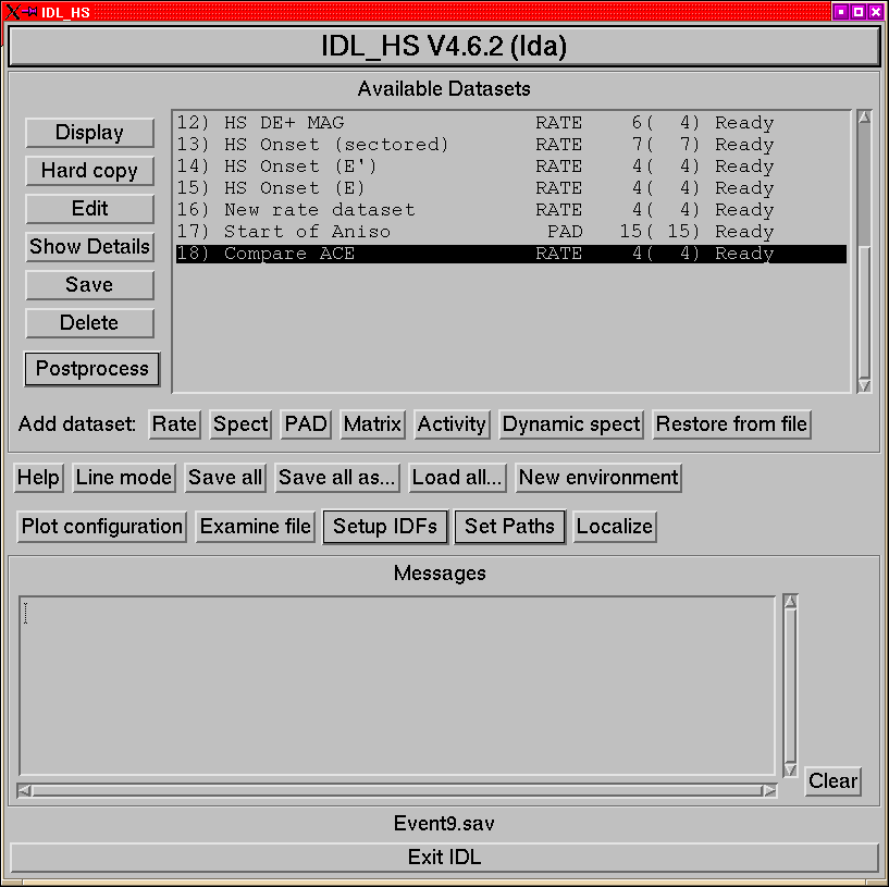
The top-level menu is very different from the old versions. It serves as an interface to defining datasets and also to setting global properties. The appearance of this menu after defining and displaying several datasets is shown in Figure 1.

**Figure 1:** The main IDL_HS menu, with several datasets defined.
$\resizebox*{0.75\columnwidth}{!}{\includegraphics{pics/main-new.eps}}$

At the top of the menu is a listbox which has a list of all the currently defined datasets and their status. The items in each line are:

An index number
The name of the dataset.
Its type, (one of RATE, PAD, SPECT, MATRIX or XFLARE).
The number of streams defined in that dataset. The number that are flagged to be displayed follows in parentheses.
Its status, this is one of:

Incomplete:

Either it doesn't have a time range, or it has no streams.

Not Ready:

The dataset is fully specified, but the data have not been read.

Raw:

The data have been read, but not processed.

Ready:

The data have been read and processed.

Immediately below this are three groups of buttons

to perform basic operations on the current dataset.
to define new datasets.
to make global settings.

The text widget below this is the window in which messages from IDL_HS are displayed.

Finally right at the bottom is a button to exit from IDL.

5.1 Operations on the current dataset

An important concept in the IDL_HS version 4 is that of the current dataset; all dataset operations are carried out on the current dataset.

The various buttons in the second group allow you to quickly perform various common operations on the current dataset:

Display: Plot the current dataset to the screen. If necessary the dataset will be read and data processing carried out.
Hard Copy: Display the dataset to the PostScript device and then revert to X-windows display.
Edit: Open the dataset menu. This can also be opened by double-clicking on the dataset's line in the dataset list.
Show Details: Display a summary of the dataset and its streams.
Save: Save the dataset to an IDL save file. The dataset can then be restored using the ``Restore DS from file'' button. (This is the easiest way to make a copy of a dataset). Please note that the underlying structure definitions may change between versions, normally changes between micro-versions (e.g. 4.1.0 to 4.1.1) should be OK.
Delete: Self explanatory.
Postprocess: This is a pulldown menu for such operations as spectral exponent calculations. The list is dependent on the type of dataset currently selected. It always contains at least an option to mark positions, and to add ``markers'' to the plot.

5.2 To create a new dataset

From the main menu, click on the appropriate new-dataset button. If an existing dataset in the dataset list is selected, then properties such as time range, HISCALE & EPAM archive types etc. will be inherited from that dataset (basically those things that were common to all programs in earlier versions).

When you do this, you will get the dataset menu which allows you to set the various properties of the dataset. Most of these should be familiar to those users who have used earlier versions of IDL_HS. The details of the specific dataset classes are described later in this document.

It is also possible to restore a previously-saved dataset (in IDL SAVE format). To do this, click on the "Restore dataset" button, this will produce a menu with which you can select the dataset to restore. A restored dataset also has all its streams and status flags preserved. Note that datasets saved with one version of IDL_HS may not be fully valid with a different version because of changes in the underlying data structures; this can usually be resolved by re-reading the data. As of 4.3.0, the IDL_HS version number is stored along with the dataset and a warning is generated if the version number is absent or lower than the version you are using. Saved datasets should be portable across operating systems and hardware.

5.3 Global operations

These items which form the third group of buttons in the menu allow settings that affect all datasets to be adjusted.

Help

Access the help system. If it has been installed, then the local copy is used, otherwise the version on the web is accessed.

Line mode

Destroy the menus but remain in IDL. Since all version 4 menus that do not have to be modal are non-blocking this is only a convenience to unclutter your screen.

Save all

Saves the container object and all its associated objects. This can then be restored by starting idl_hs with the command

: idl_hs -R filename

you can then pick up where you left off (even if you are on a different platform). Please note that the underlying structure definitions may change between versions, normally changes between micro-versions (e.g. 4.1.0 to 4.1.1) should be OK.

As of version 4.4, when an environment is saved, the filename is associated with the environment. If the environment has a filename, then this option uses that name without further prompting.

Save all as...

Save the container object and all its associated objects to a specified file.

Load All...

Restore an environment from a save file and delete the current one. If the current environment has been changed since it was last saved, then you will be asked whether you want to go ahead.

New environment

Create a new empty environment

Plot configuration

Set up the plot device. See p.

for detailed description.

Examine file:

A browser for HSIO files. See p.

for details.

Setup IDFs

A pulldown menu to allow you to set up the instrument definitions for all the various type of data that the program knows about. Each known data type where the IDF can be changed has its own menu called from this menu, those allow the version of the instrument information to be changed and the search path to be modified.

Set paths

A pulldown menu to allow you to set the data search paths for the various classes of data.

Localize

Change the paths, plotting options and UDS instrument lists to the local defaults. This is useful if you have imported a saved environment from somewhere else where data paths are different.

The ``Clear'' button below the message window, clears the contents of the message window. The "Exit IDL" button at the very bottom of the menu quits from IDL. The label above the Exit button shows the filename of the current environment and also whether it has been changed since the last save.

6 Rate datasets

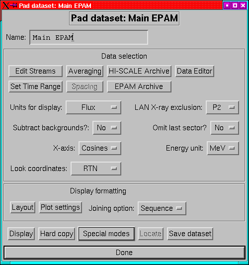
Rate datasets are used to display time-series data (historically these were just counting rates).

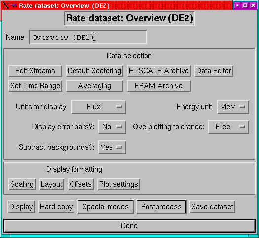
**Figure 2:** The rates dataset menu.
$\resizebox*{0.75\columnwidth}{!}{\includegraphics{pics/rate.eps}}$

The Rate dataset menu (Figure 2) offers the following settings.

Name:

A dataset can have a name which identifies it. This can be any string, and is the name which will appear on the top-level menu and also in the plot title bar.

Edit Streams:

This replaces the old channel-selection menu. This is also where to go if you want to re-arrange the order of the streams or set stream-specific options.

Set Time Range:

Set the time limits for the dataset. (p

HISCALE Archive and EPAM Archive:

Set the archive types (e.g. ULA, CUAF etc) for HISCALE and EPAM rates data. (p.

Averaging:

Set the averaging interval for the data. (p.

Default sectoring:

Choose which sector or sectors to display. (p. 12.3).

Data Editor:

Invoke the data editor on the current dataset, see page

Units for display:

Data can be plotted as flux or as count rates.

Display error bars

Decide whether to put error bars on the plot. (May not be implemented for all streams).

Subtract background

Decide whether to subtract background levels from the streams before plotting.

Energy unit

Decide whether to use keV or MeV as the energy unit.

Overplotting Tolerance:

Set the level to which the dataset should tolerate mismatched streams being overplotted. The options are:

Strict:: The streams must have an exact match of units (e.g. a Wart flux and a LEMS30 flux will not overplot).
Relaxed:: Ignore minor differences like whether energies are MeV or MeV/nuc. If there is a mismatch then the first found will be used as the label on the axis.
Free:: Anything goes! if you really want to overlay magnetic field and flux go ahead and do it (but don't blame me if you get confused).

Scaling

Bring up a menu to select various scaling options. This menu also includes the options for choosing log or linear plots and for selecting plotting against ephemeris properties.

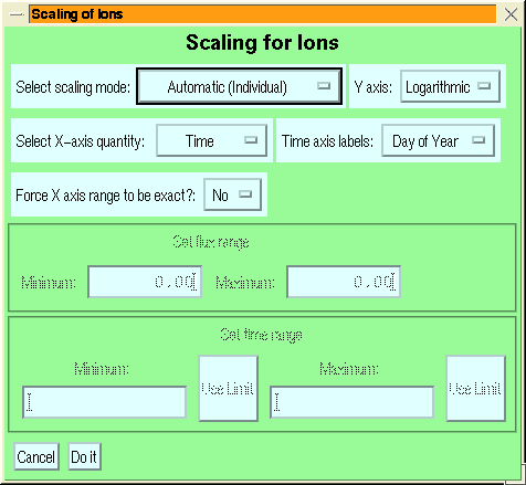
**Figure 3:** The menu to set the scaling of a rates dataset.
$\resizebox*{0.75\columnwidth}{!}{\includegraphics{pics/rate_scale.eps}}$

If a particular option is not applicable to a dataset, then the droplist for that is not displayed. The greyed-out part of Figure 3 is enabled when manual scaling is selected.

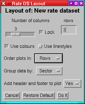
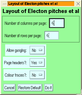
Layout

Bring up a menu (Figure 4) to choose how to lay the plot out on the page.

**Figure 4:** The menu for setting the layout of a rates dataset.
$\resizebox*{0.5\columnwidth}{!}{\includegraphics{pics/rate_lay.eps}}$

Most of the items in the menu should be obvious, however, note that:

The number of rows cannot be adjusted, there are always enough rows to show all panels in the specified number of columns.
The Lock option locks the number of columns so that if further streams are added or removed from the display then they are accomodated by changing the number of rows only, it does not stop you changing the number of columns.
The grouping option only applies when there are multiple streams with multiple sectors, then if the setting is ``group by sector'' then all the sectors of a stream are plotted on the same axes, ``group by channel'' make one plot panel for each sector. The default is group-by-sector (this is a change from 3.x where group-by-channel was the default), if the streams have different numbers of available sectors then group-by-channel is not available (however if different sectors are selected from streams with the same numbers of sectors then group-by-channel is possible, although the offsets (qv) may get confused).

Offsets

Set the offset factors between traces on a panel. These can be set, either as individual offsets for the traces or as a ratio between successive traces. Note that to clear the offsets, the best thing to do is to set the ratio to 1.0 (you need to enter a carriage return or to type something in the ratio box to make the system recognise that you've set a ratio).

Plot settings

Set a plot control specific to the dataset. By default a dataset gets its plot control information from the environment, but it is possible for a dataset to have its own set of plot controls. This menu allows you to control this option.

Display

Make a plot of the dataset. If necessary data will be read and processed.

Hard copy

Make a hard copy of the dataset. The plot device will then be switched back to X.

Special Modes:

This is a pull down menu with a number of less-used reading and display options, such as reading the data without displaying it.

Postprocessing:

This pull down menu offers the postprocessing options, e.g. a tool to measure positions on the plot and routines for calculating ratios and spectral indices.

Save

Save the dataset to an IDL save file. This can then be restored using the top-level menu's restore option. Please note that the underlying structure definitions may change between versions so that old saves may not be properly restorable.

6.1 Streams

Currently there are six main classes of stream defined,

Lan rates streams:: These are the HISCALE or EPAM rate channel plots.
Track streams:: The track rates data generated by PHAGEN, from HISCALE or EPAM data.
MFSA streams:: The 32-channel MFSA data from HISCALE or EPAM.
ULEIS streams:: The matrix rates from ULEIS.
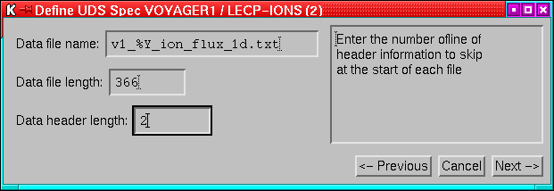
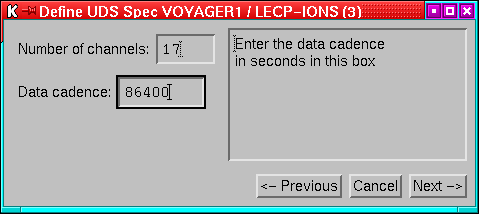
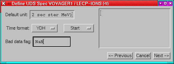
UDS streams:: Streams based on data from UDS. See Appendix A for details of how to add a new UDS stream class.
Mag streams:: Magnetic field data that have been merged into the HISCALE or EPAM rates files.

Unlike earlier versions of IDL_HS these can be freely mixed in a single plot.

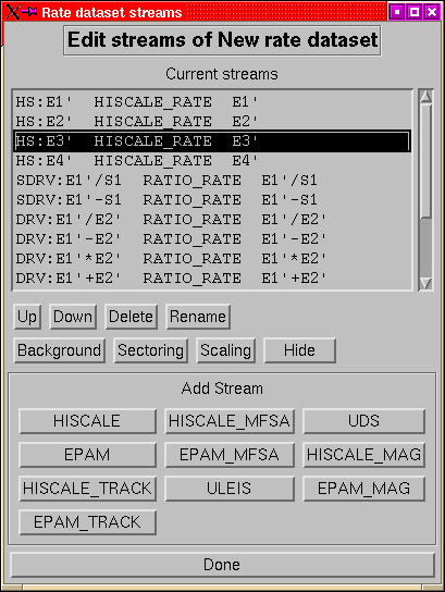
**Figure 5:** The streams editing menu for a rates dataset.
$\resizebox*{0.7\columnwidth}{!}{\includegraphics{pics/rate-streams.eps}}$

The list box at the top of the streams menu (Figure 5) Allows you to select a stream on which to work. The top row of buttons under the list all operate on the currently selected stream:

up down:: These allow you to move a stream one place up or one place down the list. If the stream is the first or last, then the inapplicable button is disabled.
delete:: Delete the currently selected stream.
rename:: Change the name of the current stream. Stream names are used to label traces in plots, however unlike dataset names they are not that vital.
background:: Change the background count rates for this stream.
sectoring:: Select the sectors to display for this stream, the default is to use the dataset settings but this option can be used to show a different selection of sectors for a particular stream.
scaling:: Set the scaling for the stream. This overrides the dataset settings. It is particularly useful for cases where one stream needs to be forced to a particular range. This setting is silently ignored when group-by-channel is in force.
hide/unhide:: Hide (or unhide) the selected stream. Hidden streams are processed just like other streams but they are not displayed. There must always be at least one unhidden stream in a dataset. Hidden streams are listed in parentheses in the stream list.

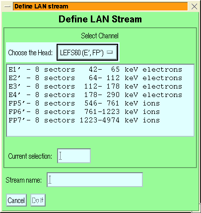
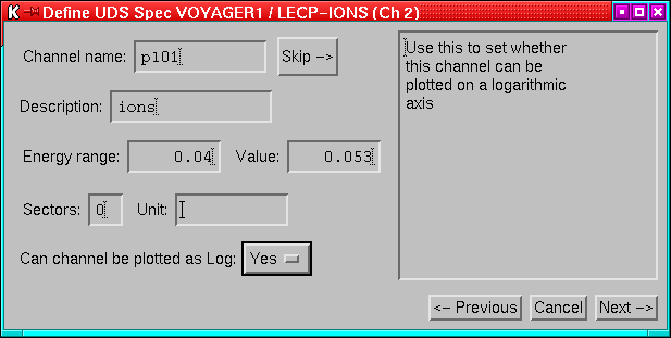
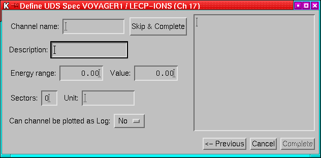
The remaining buttons allow you to add new streams. These will produce the new-stream menus for the type of stream to be added (Figure 6).

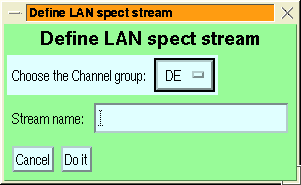
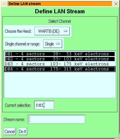
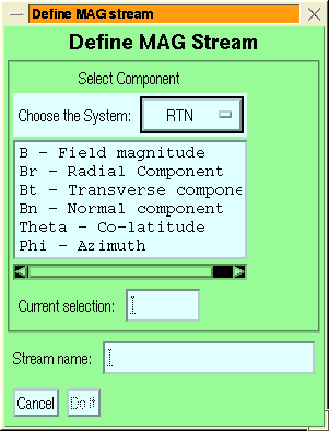
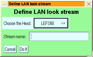
**Figure 6:** The stream-addition menus for LAN rates data (left) and MAG data (right).
$\resizebox{0.48\columnwidth}{!}{\includegraphics{pics/lan-rate-stream.eps}}$ $\resizebox{0.48\columnwidth}{!}{\includegraphics{pics/mag-rate-stream.eps}}$

The general features of the various stream definition menus are similar:

the channel group or species is selected via the top droplist
1. MFSA streams have an additional species selection to choose which species energy ranges to use in computing fluxes, so that you can look at electrons or ions with the foil channels (or any other species whose MFSA response has been characterised, but use others with caution).
2. ULEIS streams have an extra selection of ``Small'' or ``Large'' energy systems.
If desired, a range of channels can be added together by setting the second droplist to ``Range''
The channel is selected by clicking on the desired channel in the list box.
When range selection is enabled, then after clicking on the first channel, those channels which cannot be combined with it are blanked out.
Making a new selection after you have chosen a channel, replaces the previous choice.
The lists allow multiple selections using the IDL/motif multiple selection model, i.e.:
- Clicking on an item makes it the sole selection
- Shift-clicking on the item selects from the previous selection to this one.
- Control-clicking on an item toggles its selection state.
Multiple selection allows you to select several streams at one time it is not used for selecting ranges.
If you want to give the stream a name it may be entered in the text box labelled ``Stream Name''.
The ``Do it'' button confirms the selection and creates the stream, ``Cancel'' cancels the stream addition.

6.2 Postprocessing

After a dataset has been acquired, processed and displayed, there are a number of postprocessing options available.

6.2.1 Indices

This option calculates a spectral exponent between a pair of existing rate streams.

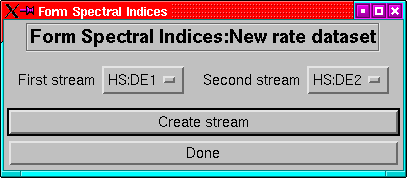
Index streams can be added to any rate stream which has been displayed (or at least acquired and processed). They are added via the ``Form indices'' options in the postprocessing menu (either on the dataset menu or the main menu); this will generate a menu to select the streams to use (Figure 7).

**Figure 7:** The menu for adding spectral indices to a rates dataset.
$\resizebox*{0.9\columnwidth}{!}{\includegraphics{pics/indices2.eps}}$

To set up an index calculation, choose the first stream of the pair in which you are interested with the left-had droplist (any streams which cannot be combined with others will not be listed), then choose the second stream with the right-hand droplist (only those streams compatible with the first will be shown), the actual order of the streams doesn't matter. To do the calculation click on ``Create Stream''. If you made the wrong selections, then just make a new pair of selections.

When you've done with generating indices, then click on ``Done'' and redisplay the dataset. If you don't want to see the original streams, then use the hide option in the edit streams menu to hide the streams you don't want to display.

The index calculation

The computation of spectral indices is an iterative process because all the channels have a finite bandwidth so that the ``effective energy'' of the channel is dependent on the spectral index. The procedure used is:

Assume the channel energies are the geometric mean of their limits (i.e. spectral index = 2).
Calculate the spectral index.
Correct the channel energies to the calculated index.
repeat 2 and 3 until either the indices aren't changing or the maximum number of iterations has been reached.

6.2.2 Calculator

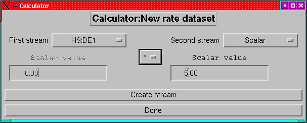
The stream calculator allows simple arithmetic operations between pairs of streams or between a stream and a scalar.

**Figure 8:** The stream calculator menu.
$\resizebox*{0.9\columnwidth}{!}{\includegraphics{pics/ratios2.eps}}$

Unlike its predecessor (including the ratios methods of versions prior to 4.4) the calculator can do more than just compute ratios (have you ever tried to generate $Br^{2}$ with ratios alone? It can be done but it is messy). The supported operations are: ratio, difference, product, sum and raising to a power (for streamscalar only). For all operations, one stream can be replaced by a scalar.

First select the stream to precede the operator using the left hand droplist (or select ``Scalar'' and enter a value in the left-hand entry field). Then select the stream to follow the operator (or ``Scalar'' and enter a value in the right hand entry field), only those streams which can be combined with the first are displayed. The operator can be set at any time.

Once a calculation has been selected, click on the ``Create stream'' button to create the new stream, note that if the second stream is a scalar and zero, then the create button is desensitized for the division operator.

When all the new streams have been defined and created, then click on ``Done''.

6.2.3 Sector ratios

Sector ratios are not dissimilar from the calculator, but instead of combining 2 streams, the operation is within a single stream and all sectors are divided by the selected sector, or one sector is subtracted from all sectors.

6.2.4 Others

The other postprocessing options are:

Write to file:

Write the dataset to an ASCII file. The format is somewhat changed from the version 3 ASCII save files.:

Line 1:: Number of streams and number of times.
Line 2:: Number of sectors in each stream.
Line 3:: A comma-separated list of the channels.
Remaining lines:: The start and end JD of each record followed by the values

If not all streams share a common time-axis then separate files are generated for each group of streams.

Locate

Allows you to use the cursor to locate positions on the plot.

Dump PNG

Allows you to dump the current graphics display to a PNG file.

Markers

Allows you to control the addition of markers to the plot.

7 PAD datasets

The PAD dataset generates plots of fluxes against pitch angle.

**Figure 9:** The main menu for PAD datasets
$\resizebox*{0.75\columnwidth}{!}{\includegraphics{pics/pad.eps}}$

Many of the settings available on the PAD dataset menu (Figure 9) are the same as those in the rates dataset menu.

Name:

A dataset can have a name which identifies it. This can be any string, and is the name which will appear on the top-level menu and also in the plot title bar.

Edit Streams:

This replaces the old channel selection menu. This is also where to go if you want to re-arrange the order of the streams or set specific backgrounds.

Set Time Range:

Set the time limits for the dataset. (p

HISCALE Archive and EPAM Archive:

Set the archive types (e.g. ULA, CUAF etc) for HISCALE and EPAM rates data. (p.

Averaging:

Set the averaging interval for the data. (p.

)

Spacing:

Set the spacing of the selected times. Thus a spacing of 1 plots every spin, while 5 plots every fifth spin. Averaging and spacing are mutually exclusive; to get say 5 minute averages and only make one plot every 15 minutes, set the spacing to 1 and use an averaging interval of 5 minutes with a spacing of 15 minutes.

Data Editor:

Invoke the data editor on the current dataset, see page

Units for display:

Data can be plotted as flux or as count rates.

LOOK direction coordinates:

Select whether to plot look-direction plots in RTN or spacecraft coordinates.

Subtract background

Decide whether to subtract background levels from the streams before plotting.

X-ray exclusion:

Set the energy level below which the Sun-sectors are excluded from LEMS30 plots.

X-axis:

Select whether to plot against cos(pitch-angle) or against pitch-angle.

Energy unit

Decide whether to use keV or MeV as the energy unit.

Layout

Bring up a menu to choose how to lay the plot out on the page.

**Figure 10:** The menu for setting the layout of a PAD dataset.
$\resizebox*{0.7\columnwidth}{!}{\includegraphics{pics/pad-lay.eps}}$

The ganging option allows you to control what happens when there are more rows available in the layout than panels. If ganging is enabled, then (for example) if there are only 2 panels and 6 rows then there will be 3 ranks of plots running across the page or screen.

Plot settings

Joining:

Select how to join up the sectors. The possibilities are:

None: don't join them up at all.
Sequence: Join the sectors 1-8 and then join 8 to 1 to form a loop.
Sorted: Sort the sectors into pitch-angle order and then join them.

Display

Make a plot of the dataset. If necessary data will be read and processed.

Hard copy

Make a hard copy of the dataset. The plot device will then be switched back to X.

Special Modes:

This is a pull down menu with a number of less-used reading and display options, such as reading the data without displaying it.

Locate:

Allows you to locate features on the plots interactively.

Dump PNG

Allows you to dump the current graphics display to a PNG file.

Save

7.1 Streams

The selection and organization of streams is rather more complex than is the case for rates datasets, as the streams are organized into panels.

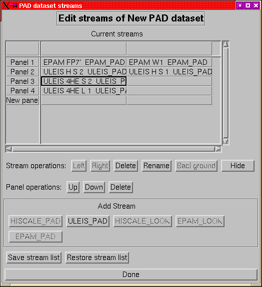
**Figure 11:** The menu for adding streams to a PAD dataset.
$\resizebox*{0.9\columnwidth}{!}{\includegraphics{pics/pad_stream.eps}}$

The table widget displays the current streams and allows you to select streams and panels for operations. When the menu is opened for the first time on a new dataset, it contains a single cell, as streams are added it is expanded.

To add a new stream to the dataset, you must first select the panel to which it is to be added (the last row of the table is always headed ``New panel'' and will create a new panel when a stream is added to it) by clicking in a cell of the panel. If you select an existing panel, then only one of the add stream buttons will be available--the one for the class of stream already represented in the panel. There are two main type of stream in a PAD dataset:

PAD streams:

The normal type of stream which shows the flux of the various sectors of a channel as a function of pitch angle. In a panel of PAD streams, the first stream sectors are indicated by the numbers 1-8, the second by the letters A-H, the third by s-z, the fourth by j-q and the fifth by various punctuation symbols (in the unlikely event of having more than 5 streams in a channel, the pattern is repeated). PAD panels are plotted as normalized values, with the peak flux indicated on the plot.

**Figure 12:** Menus for selecting streams for a PAD dataset, left - PAD streams, right - Look-direction streams.
[PAD stream selector] $\resizebox{0.48\columnwidth}{!}{\includegraphics{pics/pad-pad.eps}}$ [Look direction selector] $\resizebox{0.48\columnwidth}{!}{\includegraphics{pics/pad-look.eps}}$

LOOK streams:

A look-direction plot shows a sky map with the directions of the various sectors and the direction to the Sun and of the magnetic field indicated (by a circle and an asterisk respectively).

The menus for adding PAD streams are very similar to the corresponding rates stream menus (Figure 6) except that there is no range option and no multiple selection. The LOOK stream menu just offers a selection of heads.

Although it is in principle possible to mix HISCALE, EPAM and ULEIS data in a single dataset (although not within a panel) this can only be done if averaging is requested as the layout engine for PAD datasets requires that all streams share a common time axis.

In addition to adding channels singly, it is also possible to save a list of channels and the use the file to add a group of channels all at once. These are done with the save and restore stream list buttons. If there are already streams present when a restore is done, then the new channels are added to the existing list.

The format of the stream list is one line per panel, with a stream type descriptor first followed by a list of channels, e.g.:

EPAM_PAD E1' E1 DE1

EPAM_PAD E4' DE4

EPAM_PAD P2' P2

EPAM_PAD P4' P4

EPAM_PAD P6' P6 FP6' FP5

EPAM_PAD P8' P8

EPAM_LOOK LEFS60 LEMS120 LEFS150 LEMS30

Other stream and panel operations

In addition to the stream adding menus, there are several other operations that can be performed:

8.1.1 Stream operations:

These are available if a single cell is selected:

Left Right:: Move the stream earlier or later in the panel. This will affect the choice of symbol to indicate its sectors and (if enabled) the colour in which it is plotted.
Delete:: Remove the stream
Rename:: Change the descriptive name of the stream.
Background:: Change the background rates of the stream.
Hide/Unhide:: Hide (or unhide) the selected stream. Hidden streams are processed just like other streams but they are not displayed. There must always be at least one unhidden stream in a dataset. Hidden streams are listed in parentheses in the stream list.

Panel operations

These are available if the selection is confined to a single column (panel).

Up Down:: Move the panel earlier or later in the list of panels.
Delete:: Delete the entire panel.

Limitations

At present we do not have the ability to make PAD plots of MFSA or Track data as these do not have magnetic field merged in and the time resolution is not good enough to make meaningful pad plots.

ULEIS look plots are not supported as: firstly; there is no easy way to get the coordinate transforms and secondly; they can easily be deduced from the EPAM LEFS60 look plots.

To make ULEIS PAD plots, you must have the ACE field data in ``UMAG'' format (from DKB200:[EPAM.DATA] on epam.ftecs.com) but renamed to amagyyddd.dat (to avoid confusion with the Ulysses field data). These directory with these files needs to be in the UDS search path⁴.

7.2 Postprocessing

At present the only postprocessing options for PAD datasets are the locator tool, the screen dump, and the marker tool.

8 Spect Datasets

Spect datasets display particle energy spectra.

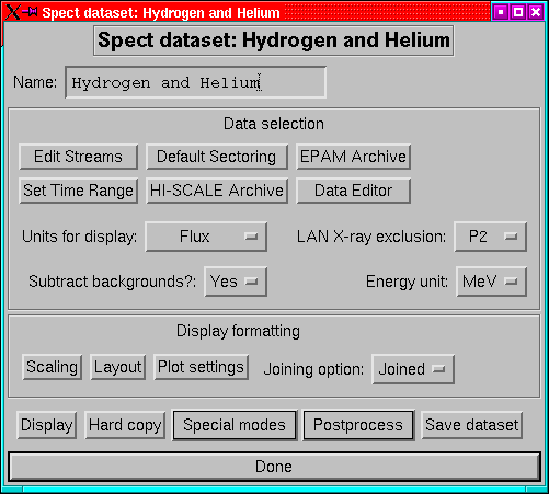
**Figure 13:** The main menu for a spect dataset.
$\resizebox*{0.75\columnwidth}{!}{\includegraphics{pics/spect.eps}}$

As is clear from Figure 13, the spect dataset menu is a bit simpler than that for rates or PAD datasets.

Name:

A dataset can have a name which identifies it. This can be any string, and is the name which will appear on the top-level menu and also in the plot title bar.

Edit Streams:

This replaces the old channel selection menu. This is also where to go if you want to re-arrange the order of the streams or set specific backgrounds.

Set Time Range:

Set the time limits for the dataset. (p

HISCALE Archive and EPAM Archive:

Set the archive types (e.g. ULA, CUAF etc) for HISCALE and EPAM rates data. (p

)

Default sectoring:

Set the default sector selection for the dataset. (p.

Data Editor:

Invoke the data editor on the current dataset, see page

Units for display:

Data can be plotted as flux or as count rates.

Subtract background

Decide whether to subtract background levels from the streams before plotting.

X-ray exclusion:

Set the energy level below which the Sun-sectors are excluded from LEMS30 plots. For MFSA plots the M channels have exclusion up to the same energies.

Energy unit

Decide whether to use keV or MeV as the energy unit.

Scaling:

Set whether to scale plots manually or automatically.

Layout

Bring up a menu to choose how to lay the plots out on the page.

Plot settings

Joining:

Select how to join up the channels. The possibilities are:

Limits:: Draw horizontal error bars to show the width of the channels in energy
Join:: Draw a polyline between the energy centres of the channels
Both:: Do both of the above.

Display

Make a plot of the dataset. If necessary data will be read and processed.

Hard copy

Make a hard copy of the dataset. The plot device will then be switched back to X.

Special Modes:

This is a pull down menu with a number of less-used reading and display options, such as reading the data without displaying it.

Postprocessing:

Allows you to run the locator tool, the screen dumper or save the data to an ASCII file.

Save

8.1 Streams

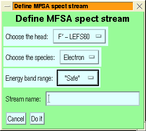
**Figure 14:** The stream addition/modification menu for spect datasets: upper - LAN data, lower - MFSA data.
$\resizebox{0.45\columnwidth}{!}{\includegraphics{pics/lan_spect_stream.eps}}$ $\resizebox{0.45\columnwidth}{!}{\includegraphics{pics/mfsa_spect_stream.eps}}$

Like PAD datasets, spect datasets have their streams organized into panels, thus the stream menu is rather similar to that of a PAD dataset.

To add a new stream to the dataset, you must first select the panel to which it is to be added (the last row of the table is always headed ``New panel'' and will create a new panel when a stream is added to it) by clicking in a cell of the panel. Unlike PAD datasets, however, stream classes can be freely mixed. The types of stream are:

spect:: (these are class lan_spect) spectra derived from the LAN rates channels (including the various WART channels). Unlike version 3 and before, the FP and E channels of the LEFS channels are treated separately.
comp:: (class comp_spect) spectra of specific species derived from TRK data.
MFSA:: 32 channel spectra from the MFSA records.
ULEIS:: Spectra generated from the ULEIS matrix rates data.

In each case the channel selection menu is a simple droplist selector, and a name box. For ULEIS streams you also need to select the energy system, and for MFSA streams the species to assume.

8.1.1 Stream operations:

These operations are available when a single stream has been selected in the table:

Left Right:: Move the stream earlier or later in the panel (effectively this only changes the colour used for it and the order of items in the title and the key).
Up Down:: Move the stream to an earlier or later panel. (At present it is not possible to move a stream into the new panel). When a stream is moved to a new panel it is added as the last stream in the panel.
Sectors:: Set the sectors to be displayed for the stream. The default is taken from the dataset setting.
Delete:: Remove the stream.
Rename:: Change the name of the stream
Background:: Adjust the background levels of the stream.
hide/unhide:: Hide (or unhide) the selected stream. Hidden streams are processed just like other streams but they are not displayed. There must always be at least one unhidden stream in a dataset. Hidden streams are listed in parentheses in the stream list.

8.1.2 Panel operations:

These are available if the selection is confined to a single column (panel).

Up Down:: Move the panel earlier or later in the list of panels.
Delete:: Delete the entire panel.

8.2 Postprocessing

Spectral datasets support the computation of sector ratios and differences, and arithmetic operations with one stream and a scalar. Since no 2 streams have the same energy bounds, it is not meaningful to allow operations between streams.

There are also options to write the dataset to an ascii file, and the locator, screen dump and marker tools are available.

8.3 Colours in spect datasets

In spect datasets, where there may be multiple multi-sectored streams, a decision has to be made as to how to allocate colours. The scheme used is this.

If all the panels have just one stream then colours are allocated by sector. With black for sector averages, red for sector 1 etc. If plot headers are in use a key is placed at the bottom of the plot.
If some panels have multiple streams, then the colours are allocated by stream and all the sectors are done in one colour. The key is then placed on the individual panels.

9 Dynamic Spectrum Datasets

A dynamic spectrum dataset is a sort of hybrid of a rate dataset and a spect dataset.

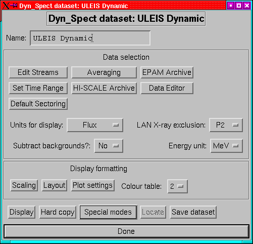
**Figure 15:** The main menu for a dynamic spectrum dataset.
$\resizebox*{0.75\textwidth}{!}{\includegraphics{pics/d_spect.eps}}$

The main menu is shown in Fig 15, as will be apparent it's pretty similar to that for spectrum datasets.

Name:: A dataset can have a name which identifies it. This can be any string, and is the name which will appear on the top-level menu and also in the plot title bar.
Edit Streams:: This replaces the old channel selection menu. This is also where to go if you want to re-arrange the order of the streams or set specific backgrounds.
Set Time Range:: Set the time limits for the dataset. (p ).
HISCALE Archive and EPAM Archive:: Set the archive types (e.g. ULA, CUAF etc) for HISCALE and EPAM rates data. (p )
Default sectoring:: Set the default sector selection for the dataset. (p. ).
Data Editor:: Invoke the data editor on the current dataset, see page .
Units for display:: Data can be plotted as flux or as count rates.
Subtract background: Decide whether to subtract background levels from the streams before plotting.
X-ray exclusion:: Set the energy level below which the Sun-sectors are excluded from LEMS30 plots. For MFSA plots the M channels have exclusion up to the same energies.
Energy unit: Decide whether to use keV or MeV as the energy unit.
Scaling:: Set whether to scale plots manually or automatically. Also selects whether log or linear scales are to be used, and whether to smooth the plot in energy and/or in time.
Layout: Bring up a menu to choose how to lay the plots out on the page.
Colour table:: Select a colour table for the display. 0 is the greyscale table. For PostScript output, if colour is not enabled, then this is ignored and greyscale is used.
Plot settings: Set a plot control specific to the dataset. By default a dataset gets its plot control information from the environment, but it is possible for a dataset to have its own set of plot controls. This menu allows you to control this option.
Display: Make a plot of the dataset. If necessary data will be read and processed.
Hard copy: Make a hard copy of the dataset. The plot device will then be switched back to X.
Special modes:: This is a pull down menu with a number of less-used reading and display options, such as reading the data without displaying it.
Locate:: Interactively mark positions on the plot.
Dump PNG: Allows you to dump the current graphics display to a PNG file.
Save: Save the dataset to an IDL save file. This can then be restored using the top-level menu's restore option. Please note that the underlying structure definitions may change between versions so that old saves may not be properly restorable.

9.1 Streams

The organization of the streams of a dynamic spectrum dataset is linear like that of a rates dataset, but the available channels are the same as those for a spect dataset. It is however doubtful whether the plain WART channels (W1+2 etc.) are of much use.

9.2 Postprocessing

Dynamic spectrum datasets support the locator, screen dump and marker tools.

10 Matrix Datasets

A matrix dataset is for displaying HISCALE or EPAM PHA matrix data. The nature of the data means that its behaviour is a little different from other dataset classes; in particular, a matrix dataset can only have a single stream.

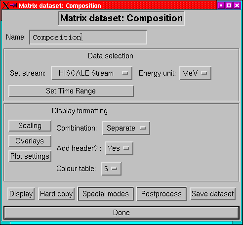
**Figure 16:** The menu for defining a matrix dataset.
$\resizebox*{0.75\columnwidth}{!}{\includegraphics{pics/matrix.eps}}$

The main components are:

Name:

A mnemonic name for the dataset.

Set stream:

Unlike other dataset classes, this doesn't bring up a new menu to select streams as there are only 2 types and the dataset is restricted to a single stream. Therefore this is a droplist item.

Energy Unit:

The energy unit for the axes of the matrix.

Set Time Range:

The familiar setting for the time limits. (p

Scaling:

Set scaling options, including selecting a subregion of the matrix.

Add header:

Do you want to put a header on the plot?

Overlays:

(Well mostly underlays actually) Select whether to indicate the locations of the WART channels, the tracks, centrelines etc.

Colour Table:

Which colour table to use? 0 is greyscale table.

Combination:

There are 3 possibilities:

Separate: means show the individual matrices and then ask the user before advancing.
Sum: means add them all up (except for the 4-fold sum matrices). This is suitable for matrices with total counts in them (the usual case).
Average: means average the matrices together (weighting the regions by their accumulation times). Suitable for the rarer count rate matrices.

Plot settings

Display

Make a plot of the dataset. If necessary data will be read and processed.

Hard copy

Make a hard copy of the dataset. The plot device will then be switched back to X.

Special Modes:

This is a pull down menu with a number of less-used reading and display options, such as reading the data without displaying it.

Postprocessing:

Allows you to run one of the locator tools or operate on histograms, or to dump the screen.

Save

10.1 Postprocessing

Matrix datasets support the regular locator tool and also a detailed locate which returns the species, energy and counts for the pixel selected.

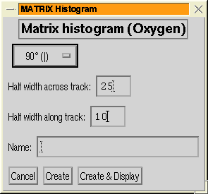
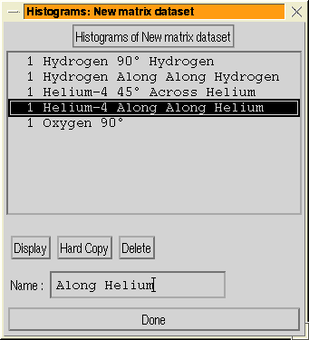
It is also possible to compute histograms either along or across tracks. Histograms are attached to the dataset in a similar way to streams, however they are not really streams (despite inheriting the generic_stream class).

New histograms are generated via the ``Histogram'' option of the Postprocessing menu. This first asks you to select a centre point for the histogram, when you have done this, you will then see the histogram options menu (Figure: 17 (left)).

**Figure 17:** The histogram menus for a matrix dataset. Left: the menu for defining a histogram; Right: the menu for displaying existing histograms.
$\resizebox{0.45\columnwidth}{!}{\includegraphics{pics/mk_histogram.eps}}$ $\resizebox{0.45\columnwidth}{!}{\includegraphics{pics/ed_histogram.eps}}$

The histogram can either be made cutting across the track, or it can be made along the track. For histograms across the track the length and width can be specified.

To (re-)display an existing histogram, you should select the ``Edit histograms'' option with allows you to display histograms, make hard copy or delete them via the histogram editing menu (Figure: 17 (right)).

In addition, matrix datasets also support the marker tool.

11 Activity Plots

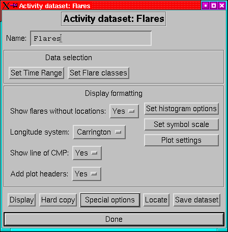
Activity plots are plots of X-ray flares as a function of time and longitude. The version in idl_hs version 4 is considerably more sophisticated than that in version 3, in that it now supports a choice of Bartels, Carrington and geocentric rotation systems and allows the generation of histograms of flare counts.

**Figure 18:** The main menu for creating activity plots.
$\resizebox*{0.9\columnwidth}{!}{\includegraphics{pics/flare.eps}}$

The main menu (Figure: 18) follows the pattern of other dataset classes with:

Name:

Set a mnemonic name for the dataset, which will appear at the top of the plot if headers are selected.

Set Time Range:

Set the time limits for the dataset. (p

)

Set Flare Class:

Brings up a menu to allow you to set the lowest intensity flare to be shown. There is also an option to set the flare class which would have a zero-sized symbol if plotted.

Show flares without locations:

Select whether flares with no optical counterpart should be plotted in a column to the left of the main plot.

Add plot headers:

Select whether to add headers to the plot.

Rotation system:

Select between Bartels (27.0 day) and Carrington (27.2753 day) rotation systems, or the raw positions relative to CMP.

Set histogram options:

Brings up a menu to select the binsize for two histograms.

A longitude histogram, showing the number of flares in each longitude bin. This will be plotted underneath the main plot, sharing a common longitude axis.
A time histogram, showing the evolution of the flare rate through the plot. This is plotted to the right of the main plot, and shares a time axis.

Show line of CMP:

Draw a dashed line showing the longitude of central meridian on the plot. This is only useful on plots with relatively few rotations.

Set symbol scale:

Set the scaling of the symbols relative to the default symbol size. Just try values till your plot looks right.

Plot settings

Display Data:

Do just that, generate the plot; reading and processing the data as needed.

Hard Copy:

Make a PostScript version of the plot.

Special modes:

A pulldown menu to select other less-used display options and also the post-processing menu.

Locate:

Interactive tool for determining positions on the plot.

Dump PNG

Allows you to dump the current graphics display to a PNG file.

Save Dataset:

Save the dataset to an IDL save file.

11.1 Postprocessing

The only postprocessing supported for activity datasets are the locator, screen dump and marker tools. Note that the marker tool applies only to the main panel not any attached histograms.

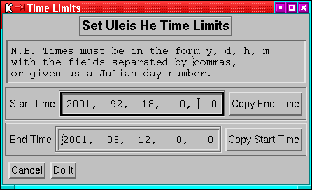
12 Settings common to several dataset classes

12.1 Time range

Applies to all datasets.

In the times menu, times may be entered either as year, day, hour, minute, second, or as a julian day number.

**Figure 19:** The menu for entering the time range for a dataset.
$\includegraphics{pics/time.eps}$

If a single number greater than 2 million is entered, the it is assumed to be a julian day, if multiple numbers are used, then a year, day etc. form is assumed. If a single number less than 2 million is entered, it is assumed to be a year (with a warning). If a 2-digit year is used it is assumed to be in the range 1950 to 2050.

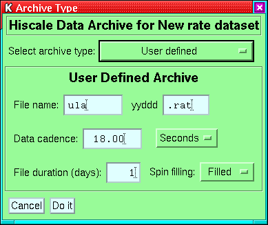
12.2 Archive types

Applies to RATE, SPECT, PAD and DYN_SPECT datasets.

**Figure 20:** The menu for setting HISCALE archives.
$\includegraphics{pics/archive.eps}$

The basic pre-defined archives are selected via the ``Select archive type'' droplist at the top of the menu. If you are using some special type of data, then you will need to select ``User defined'' and then set the various fields. The defaults are taken from the previously set archive type. A couple of points to note: (1) The file duration should be set to the maximum possible for the file class, (2) The spin filling refers to whether all the spin groups are used (as in ULA and CUAF files) or only the first spin group (as in UAF files).

Since it is now possible to display HISCALE and EPAM on the same plot, the selections are independent for the two instruments.

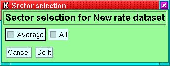
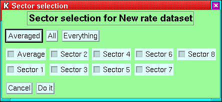
12.3 Sectoring

Applies to RATE, SPECT and DYN_SPECT datasets.

**Figure 21:** The menus for sector selection. The upper menu is used when no streams are defined, or if the streams have different numbers of sectors. The lower version is used when all streams have the same number of sectors (the actual number of toggle buttons depends on the number of sectors).
$\resizebox{0.7\columnwidth}{!}{\includegraphics{pics/sectors1.eps}}$ $\resizebox{0.7\columnwidth}{!}{\includegraphics{pics/sectors2.eps}}$

For datasets where all the streams have the same number of sectors, an arbitrary combination of sectors can be selected (e.g. if you really want to you can plot the average, sector 1 and sector 3). If the selected streams have differing numbers of sectors, then only sector averages or all sectors can be selected at the dataset level (however detailed selections can be made for the individual streams--the control for this is very similar to that for datasets). If you try to set sector selection before you have attached any streams to the dataset, then you will only have the choice of average or all. At present there is no phase-angle sorting of the sectors.

The ``All'' button in the menu selects all the individual sectors, and NOT the average. The ``Everything'' button selects all the individual sectors and the average.

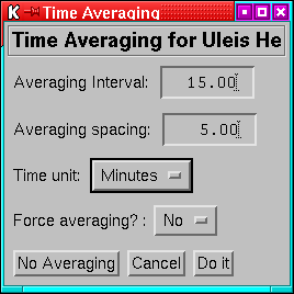
12.4 Averaging

Applies to RATE, PAD and DYN_SPECT datasets.

**Figure 22:** The menu for setting averaging intervals. The settings here will generate overlapping 15-minute averages every 5 minutes.
$\includegraphics{pics/average.eps}$

This allows you to set an averaging interval for the current dataset.

As with earlier versions, overlapping averages are possible. If the spacing is set to zero, that is equivalent to setting it equal to the averaging interval (i.e. non-overlapping averages). Unlike earlier versions ``gappy'' averages are possible; this is likely to be of most use in PAD datasets where (for example) using hourly averages would smear out what you wanted to see, but 5-minute averages would overwhelm you with data; in that case 5-minute averages every hour may be what you need.

If the averaging interval is less than the cadence of the datset, averaging will not take place, unless the forced average option is selected.

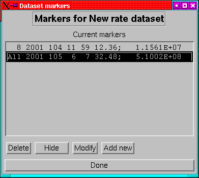
12.5 Markers

Markers are user-defined labels that can be added to any dataset. They can be used (for example) to accurately place timing marks on a plot or to place a box around a feature to which attention is to be drawn.

A marker has a number of vertices, and optionally a text string. The details vary according to the dataset class, but in essence a marker can appear on any or all panels. At present; in activity datasets, markers are only supported in the main panel, and they are not available on matrix histograms.

**Figure 23:** The marker editing menu for a dataset.
$\includegraphics{pics/ds_marker.eps}$

The dataset markers menu (Figure 23) is accessed from the markers item in the postprocessing menu. This lists defined markers by panel, location of first vertex and (if applicable) text string. A marker can be deleted, hidden or edited or new markers can be added.

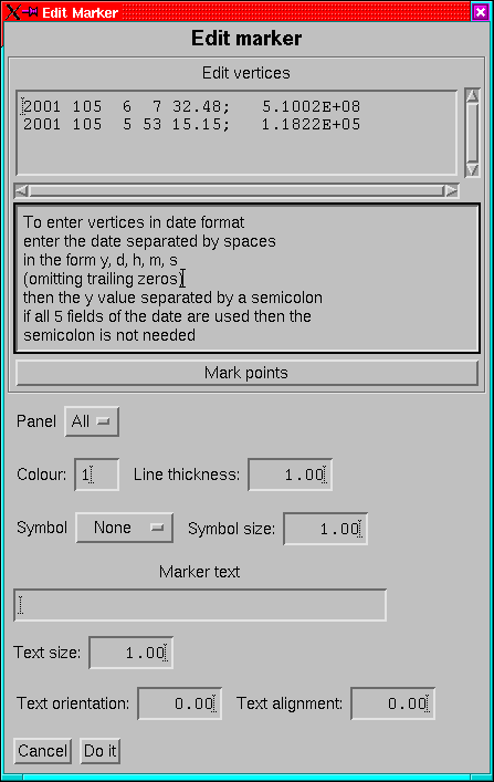
**Figure 24:** The menu for editing an individual marker.
$\resizebox*{0.6\columnwidth}{!}{\includegraphics{pics/marker.eps}}$

The modify and ``add new'' options will generate the marker menu (Figure 24). For most datasets, vertices can either be entered manually in the text box (when an axis is a time-axis, then the coordinate can be entered in year, day, h,m,s format by follwing the displayed instructions) or marked using the locator tool (this is not possible for PAD or MATRIX datasets as the page number cannot be determined, thus the panel is not uniquely defined).

When applicable, the panel to which to add the marked can be set. For SPECT and PAD datasets, this corresponds to the panel number in the dataset. For RATE and DYN_SPECT datasets, the panel is defined in terms of the order in which they are plotted. In either case, if the panels are re-arranged the markers do NOT move to the new panels. For PAD and MATRIX dataset, there is also a time panel setting which can likewise refer either to a single time panel (page for MATRIX, column for PAD) or everything.

The colour, thickness, symbol and symbol size are just the standard IDL settings (colour of course using the IDL_HS colour table). The vertices are always joined even when a symbol is used.

When text is added to the marker then it is located at the first vertex and the remainder are joined. The size, orientation and alignment can be set. The colour is the same as the line joining the other vertices.

13 The data editor

The data editor is a tool for making simple edits to the actual values in the raw data. The reason for this is to allow the user to remove closed-cover calibration features, telemetry problems etc. It operates on RATE, SPECT, PAD and DYN_SPECT datasets; MATRIX datasets generally have too few points and are also generally used a a qualitative display.

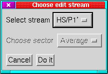
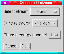
**Figure 25:** The menus for selecting the stream to work on in the data editor. Left: for rate or PAD datasets, Right: for SPECT or DYN_SPECT datasets.
$\resizebox{0.4\columnwidth}{!}{\includegraphics{pics/edit-rate-c.eps}}$ $\resizebox{0.4\columnwidth}{!}{\includegraphics{pics/edit-spect-c.eps}}$

The data editor is invoked by clicking the ``Data Editor'' button on the dataset main menu. Do not confuse this with ``Edit Streams'' which is to add or delete streams from the dataset. When you call up the editor, you will first be asked which stream from the dataset you wish to use as the template (Figure 25). You need to select which stream and in the case of sectored streams which sector as well. For Spect datasets you also need to select which energy channel to use.

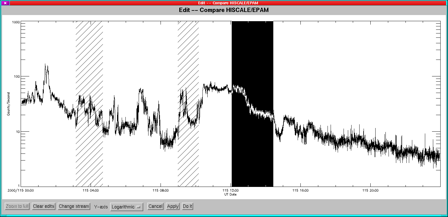
**Figure 26:** The main data editor window with 2 committed edits and a region selected.
$\resizebox*{1\columnwidth}{!}{\includegraphics{pics/editor.eps}}$

When you have selected a stream, it is displayed and you can make the edits.

On the display canvas, the mouse buttons have the following effects:

Button 1:

(Usually left button), starts a selection. The location of the pointer is translated to a time and this marks the edit start. Motion events on the a canvas are enabled, so that when the mouse is moved, the area between the marked location and the current pointer position can be shown inverted. If the left button is clicked a second time, the previous start location is forgotten and a new selection is started.

Button 2:

(Usually centre button), cancels a selection.

Button 3:

(Usually right button), completes a selection. This sets the current pointer location as the end point of the selection. The edit-type menu is then displayed to determine the edit type.

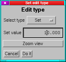
**Figure 27:** The menu for choosing the type of edit to make.
$\resizebox*{0.7\columnwidth}{!}{\includegraphics{pics/edit-type.eps}}$

This menu (Figure 27) allows you to select the type of edit or to zoom the view to the region selected. There are 4 type of edit:

Cut:: Simply remove the data for the selected interval and leave a gap in the time-series (For most purposes this is the most suitable edit).
Zero:: Set the rates to zero through the selected interval.
Set:: Set the rates to a user-selected value through the selected interval.
Add:: Add a user-selected value to the rates in the selected interval.

After an edit has been committed, the region is marked by a hatched box. Edits are not actually made at this stage.

If you click on the zoom button, then the region of the selection is expanded to fill the window. The cancel button causes the edit to be abandoned.

Other_buttons:

At present buttons 4 & 5 (wheel mouse wheel rotations) are ignored.

The following operations are available via the buttons at the bottom of the panel:

Zoom to full:: Revert to showing the entire time range of the stream.
Clear edits:: Delete the list of edits.
Change Stream:: Change to a different stream. This clears all edits made up to this point and reverts to the stream selection menu.
Y-axis:: Choose whether to show the stream on a log or a linear scale. Not available for streams which cannot be plotted on a log scale (e.g. magnetic field components).
Cancel:: Exit the editor without applying the currently committed edits.
Apply:: Apply the currently committed edits, and continue editing. Note that once edits have been applied they cannot be undone.
Do it:: Apply the currently committed edits and exit the editor.

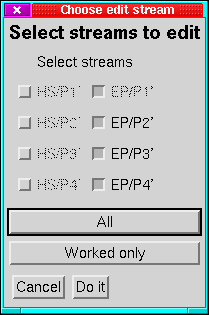
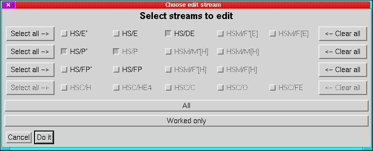
**Figure 28:** The menus for selecting which streams to edit. Left: Rate dataset, Right: SPECT or PAD dataset.
$\resizebox{0.25\columnwidth}{!}{\includegraphics{pics/edit-rate.eps}}$ $\resizebox{0.7\columnwidth}{!}{\includegraphics{pics/edit-spect.eps}}$

On selecting ``Apply'' or ``Do it'' you will then be asked which streams the edits should be applied to. There are two distinct menus (Figure 28) depending on whether the dataset is divided into panels or not.

In either case, only those streams sharing a raw time axis with the stream on which you made the selections can be modified. The streams to modify are selected by the toggle buttons in the menu, all streams are shown but only those with the correct time axis can be selected. The stream on which the edits were defined cannot be deselected. The ``All'' and ``Worked only'' buttons below the stream list allow you to select all applicable streams or only the one on which you made the selection.

For hierarchical datasets (SPECT and PAD) the toggles are layed out with one row for each panel of the display. In addition there are two columns of buttons; one on the left ``Select all ->'' which selects all applicable streams in that panel, and one on the right ``<- Clear all'' which allows you to deselect all streams in the panel (other than the one you made the selections on). For PAD datasets it is not a good idea to apply edits to only a subset of streams if the edits include cuts (zeros, sets and adds are OK) because this will break the time-axis matching and make the dataset undisplayable without averaging.

The ``Cancel'' and ``Do it'' buttons have their normal effects.

WARNING: If you use the editor before you have created a regular plot window, you may find that the visual properties that you selected are not honoured, and worse than that they will be broken until you exit IDL and re-enter. This problem may have been resolved in IDL 5.4 (I've had apparently contradictory results) but is present in 5.2. This is particularly the case if you select an undecomposed true colour visual (idl_hs -T or HS_BITS=24). The only fix for this is to display a dataset before editing.

14 Other parts

14.1 Plot settings

Normally the plot settings are global to the environment, but a dataset can have its own plot settings if needed. The plot settings controlled from the main menu ``Plot configuration'' button is the global one, those controlled from the dataset menu ``Plot settings'' menus are specific to the dataset. If a dataset has its own plot settings then the global settings are ignored entirely (i.e. it is not a setting by setting control).

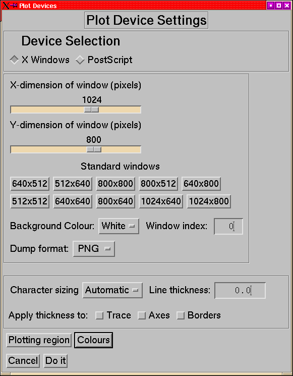
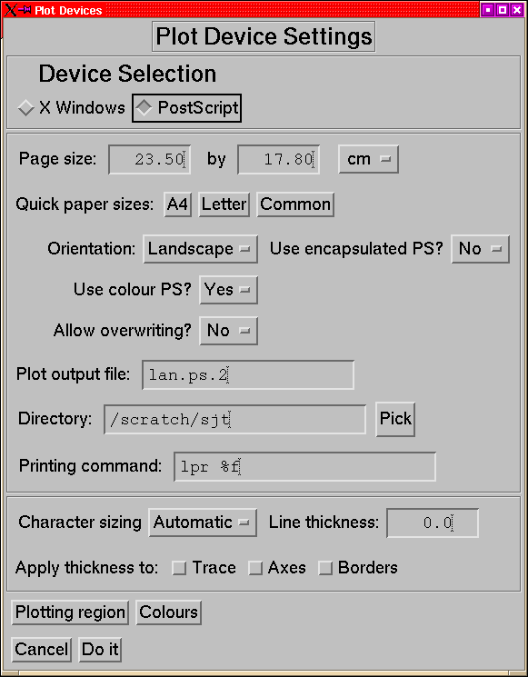
This is the tool for configuring the plot devices.

**Figure 29:** The plot setup menus for the X and PS devices.
$\resizebox{0.45\textwidth}{!}{\includegraphics{pics/plot-x.eps}}$ $\resizebox{0.45\textwidth}{!}{\includegraphics{pics/plot-ps.eps}}$

Device Selection:: Chooses whether to set up the X or PostScript output device.
``Window Sizing'' [X]: The size of the plot window for X can be set either by the sliders (which allow any size up to the current screen size) or by selecting one of the convenient standard sizes - note that for small displays the largest of these may be bigger than your screen.
Background Colour [X]: You can either plot with a black background and white lines (the IDL default behaviour) or with a white background and black lines which is often easier to look at.
Window_index [X]: Not often needed, but if you have a plot in a plot window which you don't want to overwrite then you can force IDL_HS to use a new window this way.
Page size [PS]: Set the size of the drawing area for the plot. The unit can be either centimetres or inches. The pre-defined sizes are set up to be suitable for printing on A4, US Letter or either.
Orientation [PS]: Select whether to print in landscape or portrait page orientation, if appropriate the X and Y sizes of the printing area are swapped. Note that for Encapsulated PostScript the size swap is all that happens since real landscape EPS files are a recipe for trouble.
Use colour [PS]: By default IDL uses monochrome PostScript files. This option allows you to generate colour PS files. Note that printing colour files on monochrome printers can take a VERY long time.
After plotting [PS]:: This determines the behaviour of IDL_HS after a hard copy has been generated. If this is set to retain, then the device will remain set to PS, whereas of it is set to revert, then the device is set back to X after the plot has been generated. Using the ``Hard Copy'' button on the main menu or on a dataset menu will force ``retain''
Use encapsulated PS [PS]:: This should be familiar, but when it is enabled, then the blank space in the menu is filled with another droplist offering you the choice of whether to add a pixmap to the EPS file. If you are only planning to use the EPS file for L^ATEX, LYX or xfig you do not need this, but StarOffice and other even dumber word processors need this to produce any sort of preview (and it's a pretty lousy preview too).
Allow overwriting [PS]: If you have given an explicit filename, but that file already exists, then this allows you to select whether to overwrite it or to use the default filename instead.
Plot output file [PS]: Select the name of the output file (the default is lan.ps.n where n is the lowest number that doesn't already exist.
Directory [PS]: Select the directory in which to put plot files.
Printing Command [PS]: The command to use to print a PostScript file, the token %f represents the filename. When Encapsulated PS is selected, then this is replaced by the box to select the preview command.
Character Sizing: By default IDL_HS chooses its character size by looking at how many panels there are on the plot. However if you want you can force it to use either the smaller or larger size.
Line thickness:: This line thickness option is intended as a means of making plots with bolder lines than normal for publication or presentation purposes (that is why it's here not in the dataset layout options). The thickness is specified as a floating point number which is interpreted as points in PostScript and pixels in X (therefore the results will look very different on the screen and on the page). The thickness setting can be applied to any combination of: the plot traces, the axes, and the boxes drawn around the page sections; there is no way to set 2 different non-default thicknesses⁵.
Plotting region: Brings up a menu to set what part of the window or page to use. This is probably largely obsolete and was introduced in very early versions as a number of devices didn't work too well very close to the edges.
Colours: Brings up a menu to allow you to change the colours used for coloured traces.

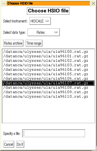
14.2 Examine File

The HSIO browser allows you to open an HSIO file and examine the contents in detail.

**Figure 30:** The menu for choosing a file for the HSIO browser.
$\resizebox*{0.7\columnwidth}{!}{\includegraphics{pics/browse_file.eps}}$

The file to look at is selected via a menu (Figure: 30) which allows you to pick a file from a list or to specify an explicit file. The files displayed in the list are controlled by the selection of the instrument and the the type of data. The selection is further limited by the time range which may be specified. For rates data an archive type may also be given. If a current dataset is defined at the time, then the time range and archive type are inherited from that.

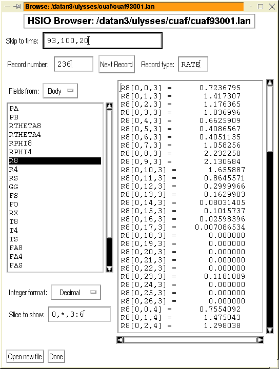
**Figure 31:** The main window of the HSIO browser tool.
$\resizebox*{0.9\columnwidth}{!}{\includegraphics{pics/browse.eps}}$

Once the file has been opened, then the main HSIO browser window is opened (Figure: 31).

The top few items in the window allow you to select which record to view. If the file has a map then the ``Skip to time'' item allows you to find a record shortly before the time you specify, if there is no map file then the option is not displayed. The record number field serves 2 purposes, firstly to indicate the current record number and secondly to allow you to go to a specific record. The next record button advances the file to the next record. The record type field is not writable but just indicates the type of the current record.

The left column of the main body of the window allows you to select which values to display. The ``Fields from'' droplist lets you choose whether to look at the record header or at the main body of the record. The list below that allows you to then select the particular field to display. The integer format allows you to select how integer fields will be displayed, this is useful because many of the housekeeping fields are actually byte values replicated 4 times so the byte display options make it possible to see what's going on. The slice allows you to select a part of the array to display, it is a standard IDL subscripting expression (the parentheses or brackets are optional, the interpreter is smart enough to decide if it needs to add them).

The ``Open new file'' and ``Done'' buttons at the bottom should be self-explanatory.

As a note to the technically-inclined, the HSIO browser is actually implemented as a dataset class, but with some restrictions: It never has any streams attached (although by inheriting the generic_dataset class it has the hooks for them), there is never a reference to it in the dataset list of the hs_container object (it does though have a reference to the container) and it is destroyed when its display window is destroyed. [In the documentation comments I've tried to refer to it as a pseudo-dataset rather than a dataset].

15 General Points

The following section is a sort of FAQ, a few random points that have cropped up along the way.

15.1 Modal Menus

When a menu is called from an object constructor it has to be modal as it is not safe to allow the constructor to return before the menu has exited. The main cases where this is used are:

The stream addition menus.
File selectors.
Alert, query and error dialogue boxes.

Note that if a pulldown menu is activated while waiting for a modal menu to appear, this is very likely to crash IDL (this is an IDL or Motif bug not an IDL_HS bug).

15.2 Backgrounds

The default backgrounds for those channels which have backgrounds defined are set in the IDF file. However when a stream is defined, then a copy is made of the background levels. This has 2 consequences:

If you change the IDF file for an instrument, the backgrounds (and most other properties) of already-defined streams will NOT be changed.
You can change the background of a particular stream individually.

The background setting tool it to be found on the stream menu of the dataset (Add/Delete stream). To access it you need to select a particular stream and then the background button will be enabled.

A. UDS data and its specification.

A..1 Introduction

Originally UDS stood for ``Ulysses Data System'', a set of summary data from each of the Ulysses instruments available from ESTEC. However the nature of the UDS formats (ASCII files with a time and then a series of data) lends itself to extension, so for the purposes of IDL_HS, UDS can be taken to mean ``User Defined Scheme''.

A..2 Specification

The UDS classes are described by a specification file, which contains the information necessary to read the data from the file.

Each line consists of a colon separated list of items.

Line1:

Is the general specification, the fields are

The spacecraft. (e.g. ULYSSES)
The instrument (e.g. COSPIN-HFT)
How many channels are there (including unused fields that must be read)
The cadence of the data in seconds
The format of the time field, recognised forms are:

YDHMS

- Year, day, hour, minute, second

YDHM

- Year, day, hour, minute

YD(H)

- Year, day, (hour) [Day is floating and hour is redundant]

JD

- Julian Day

AE

- ACE Epoch

E1950

- Seconds after 1950.0 (Ulysses epoch)

an optional /m indicates that the times are at the mid-point of the interval while /b indicates both limits are present otherwise the time is assumed to represent the start of the interval.
The unit of the values
The missing or bad data flag
Number of lines of header information.

Line2:

The filename and how long the file is:

The duration of the file in days
The filename in which the data are found. The following tokens are used: %y 2-digit year, %Y 4 digit year, %d 3-digit day, %q 1-digit quarter (1=Jan-Mar etc).

Lines3-end:

The specification of each channel, inapplicable fields (e.g. energies for magnetic field data) may be left blank.

Channel name
Lower energy bound
Upper energy bound
Description
N sectors
Unit if different from that in the header.

A channel name of DUMMY indicates values that are not used, but which need to be read. A channel name prefixed with an asterisk means the channel is not directly used but needed (e.g. quality flags).

The files are called <name>.SPEC, N.B. upper case SPEC on Unix systems. The default spec files are for all the particle and plasma datasets in the UDS plus the magnetic field files from the ACE Science Center, and the UMAG files used by MAGMERGE.

A..3 The Wizard

There is now a wizard available to generate SPEC files for UDS datasets. This can be accessed from the IDL> prompt, by giving the command

: uds_wizard

This will then generate a series of menus which will lead you through the process of defining a new UDS instrument type.

**Figure 32:** The various stages of the UDS specfile wizard.
$\resizebox{0.7\columnwidth}{!}{\includegraphics{pics/wizard1.eps}}$ $\resizebox{0.7\columnwidth}{!}{\includegraphics{pics/wizard2.eps}}$ $\resizebox{0.7\columnwidth}{!}{\includegraphics{pics/wizard3.eps}}$ $\resizebox{0.7\columnwidth}{!}{\includegraphics{pics/wizard4.eps}}$

**Figure 33:** The channel definition pages of the UDS specfile wizard. Upper: most channels; Lower: Final channel.
$\resizebox{0.7\columnwidth}{!}{\includegraphics{pics/wizard5.eps}}$ $\resizebox{0.7\columnwidth}{!}{\includegraphics{pics/wizard6.eps}}$

Figure 32 shows the 4 stages of defining the global properties of the instrument. Figure 33 shows the panel for defining the individual channels.

By default the generated spec file is saved in ${HOME}/uds_specfiles, unless an alternative has been set in the UDS_SPEC_PATH resource setting.

B. Default settings and customisation

IDL_HS version 4 has several levels of default settings for IDF files and for plot settings.

The ultimate level of fall back is the hard-coded defaults which are used if no values are found anywhere.

These values may be overridden by either a user's own resource file or by a system-wide resource file. Both of these files allow the same items to be specified. The system file is read first, followed by the user's file. Except for path settings (see below), in the case of multiple settings the last one encountered is used.

On all systems the system file is: ${IDL_HS_DIR}/Data/idl_hs.rc or equivalent. On Unix and Unix-like systems the user's file is ${HOME}/.idl_hsrc while on VMS it is HOME:idl_hs.rc.

Resource specifications are given 1 per line and have the form:

: RESOURCE = value

The resource name is not case-sensitive, but the value is. Comments begin with the hash (#) symbol. If the token ${text} is encountered in a value, then it is replaced by the value of the environment variable (for example if the string /scratch/${USER} is encountered when reading a resource file and you are user sjt, then the value will be /scratch/sjt.

Path settings are handled somewhat differently from other resources in that multiple values can be concatenated. If you want paths to be concatenated to the existing defaults, then use a + sign at the start to prepend the extra path then use ++. For example:

: HS_RATE_PATH = /data/hiscale

will set the HISCALE rates search path to /data/hiscale, whereas:

: HS_RATE_PATH = +/data/hiscale

will add /data/hiscale to the end of the existing path and

: HS_RATE_PATH = ++/data/hiscale

will add it to the beginning of the path. In either case the values may be path lists, separated by colons on Unix and commas on VMS.

B..1 rc_maker

The data directory contains a resource file template (idl_hs.rc-list) which contains the full list of resources, the types of values they can contain and default values. This can be parsed with the rc_maker procedure.

To set up a system resource file use:

: rc_maker, /system

For a user resource file use:

: rc_maker

: rc_maker, file=<filename>

if you want to check the results before replacing your file.

For each known resource value you will be presented with a menu allowing you to change the value (the default is the value currently defined or else a default defined in the template). You have the option to apply the resource in which case it will be written out to the file, or to skip it which means that it will not be written (for example if you are creating a personal file and wish to keep the system values for a particular resource).

B..2 Defined resources

The hard defaults are given in square brackets. The first group of options, should be set by the administrator in the system-wide resource file to suitable values for the local system.

HS_RATE_PATH: Search path for HISCALE rates data, should contain your usual ULA and averaged data directories. [current directory]
EP_RATE_PATH: Ditto for EPAM. [current directory]
HS_TRK_PATH: Search path for HISCALE track and PHA matrix data. [current directory]
EP_TRK_PATH: Ditto for EPAM. [current directory]
HS_MFSA_PATH: Search path for HISCALE MFSA data [current directory]
EP_MFSA_PATH: Ditto for EPAM [current directory]
ULEIS_PATH: Search path for ULEIS HDF files. [current directory]
UDS_PATH: Search path for UDS files. [current directory]
UDS_SPEC_PATH: Search path for UDS spec files (other than the standard data directory which is hardcoded in) [${HOME}/uds_specfiles]
XFLARE_PATH: Search path for X-ray flare listings. [current directory]
HS_IDF: The filename of the HISCALE IDF.DAT file. [IDF.DAT]
EP_IDF: Ditto for EPAM. [IDF-EPAM.DAT]
HS_PHA_VERSION: The PHA matrix version for HISCALE [9]
EP_PHA_VERSION: The PHA version for EPAM [11]
HS_MFSA_IDF: The filename for the HISCALE MFSA energies etc. [mfsa_energies.dat]
EP_MFSA_IDF: The filename for the EPAM MFSA energies etc. [mfsa_energies.dat]
PLOT_DIR: A directory to which to write plot files. [current directory]
PS_PRINT: The print command for spooling normal PostScript files (the token %f is used to represent the filename). [lp %f or print %f]
EPS_VIEW: The command to display Encapsulated PostScript files. Ending this with an & character will cause it to be run in the background. [gv %f &]

The remaining options will not normally need to be set in the system-wide resource file, but may be useful for users with specific preferences or requirements.

AVERAGE_UNIT: Set this to one of days, hours, minutes or seconds to set the default unit for specifying averaging intervals. [hours]
MATRIX_COLOUR_TABLE: Set the default colour table for matrix datasets. [0]
PIXMAP: Set this to yes if your X-server doesn't support backing store (typically this is a problem on older X-terminals), then IDL will use a pixmap to do the backing store. [no]
SMALL_FONTS: Set this to yes to use smaller fonts for the widgets. Useful if you have a small screen. [no]
X_BACKGROUND: The background colour for X windows window (should be black or white). [black]
X_SIZE: The size of the window in pixels, should be two integers separated by spaces. [640 512]
PS_SIZE: The size of the drawing area on the PostScript page, two floats separated by spaces. Units are specified by the PS_UNIT resource. [23.5 17.8]
PS_UNIT: The units for the PostScript page size (should be cm or inch). [cm]
PS_ORIENT: Whether the PostScript page should be landscape or portrait by default [landscape]
PS_COLOUR: Whether PostScript should be colour by default. [no]
PAD_LAYOUT: The number of columns and rows in which to layout PAD plots , two integers [6 6]
HTML_VIEWER: Viewer for HTML to view the help system [${IDL_HS_DIR}/bin/nshelp] (this script is a wrapper for the -remote option in Netscape).
SAVE_DIR: A directory to which saves and restores are to be made. The same directory is used for saving datasets and other things (such as PAD channel lists) [current directory]. Because of the way in which the file-selector widget works, it is slightly cleaner to add the trailing slash to the directory name.
QUIET: If this is set to YES then all compilation messages from IDL will be suppressed. [no]
START_MENU: If this is set to NO then the top-level menu will not be started automatically, this might be a good idea if you are regularly connecting over a slow link. [yes]

About this document ...

IDL_HS Version 4: User's Guide

This document was generated using the LaTeX2HTML translator Version 2K.1beta (1.47)

The command line arguments were:
latex2html -no_subdir -split 0 -show_section_numbers /tmp/lyx_tmpdir24851b1pYaF/lyx_tmpbuf24851EsNhj8/Uguide.tex

The translation was initiated by James Tappin on 2002-07-17

Footnotes

... data ¹: The MFSA rates and spectral data now use Doug Patterson's incident energy values in place of the old ``deposited energies''--the latter can still be used as an option.
... dataset ²: Basically everything except its channel list.
... dataset ³: Apart from UDS and MAG streams which have fixed units of display.
... path ⁴: This is a technical requirement, in that the mechanism for reading the amag files is the same as that used by UDS rate streams.
... thicknesses ⁵: It is possible that setting !p.thick at the IDL> prompt and then using another setting here could achieve this effect - I've not tried it.

James Tappin 2002-07-17