Exercise 1 - Source finding

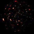
     X-ray images from XMM-Newton typically contain many point-like sources of X-rays, and an astronomer's first job is typically to locate all these sources, so that they can be checked against known astronomical objects. This exercise will take you through a step by step guide on how to find X-ray sources in the images provided in the image library. The "Lockman" data used here is the result of a long XMM observation of a region known as the "Lockman Hole". This lies in a direction where absorption of X-rays due to interstellar gas and dust is especially low, and so is a popular target for X-ray astronomers.

In what follows, new concepts will be introduced and the level of understanding will gradually be built up through a series of tasks. Problems such as noise and background will be introduced, as will a method for dealing with them.

Step 1 - opening an image

     Firstly start up Scion image. Then use the Open command in the File menu and select an image from the x-ray sources folder in the image library which you previously downloaded. If you followed the instructions in the image library page then this can be found in the images folder in the Scion image directory. The example image used is lockman_05_2.tif. It is recommended that you use this image first so that you can compare your resulting images and results with the example ones given.

Step 2 - First analysis

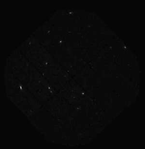
     Once the image has been loaded the first source searching phase can begin. The dark background picture elements ("pixels") in the image have high values and the bright source pixels have low values, in reality a source has a high count of photons and the background has a low count. To reproduce this in the image, you need to invert it using the Invert command in the Edit menu. Now you can see that the sources have a high value and the background has a low value. Save this image under a new name, if you are using the recommended image than call it Lockman_05_2inv.tif. Now click on Threshold in the Options menu. Set the threshold to 3 i.e. allowing all grey shades above 3 to be visible and all below 3 to be ignored. (Your image should now look like the image to the right)

Once the threshold is set, open the Analyze menu and click on Set scale. Change the units to pixels, and then click ok. In the Analyze menu still, click on Options. In the options menu check the X-Y Center box, and ensure Area is also checked, then change the Max. measurements value to 1000, and click ok. Next click on Analyze again and then click Analyze particles. Set the minimum particle size to 4 so that only particles of a significant size are counted. Finally make sure Label particles, and Reset Measurement Counter are checked, then click ok. The program will now determine the position of the particles on the screen.

(At this point it is worth mentioning what is meant by a "particle". A particle in Scion image is a region in threshold mode which is a single contiguous set of pixels which lie above the threshold. A particle is surrounded by a region which is below the threshold.)

You can clearly see that with the minimum particle size set to 4, a lot of scattered dots appear on the display, in fact you should get 868 particles.  If you had used a smaller size there would be even  more particles. Most of the particles that have been counted will not be real sources and will just be noise. You can now close this window, and you do not have to save the image.

     Noise and background are problems which even the best Charge Coupled Devices (CCDs) can not overcome. Despite this there are methods of reducing their effects on an image and the next section of the laboratory will teach you about these.
 

     An image consists of a set of detected photons, in an array of pixels. Each detected photon causes a "count" to appear in one of the detector pixels. In astronomy, we are interested in photons arriving from cosmic objects, however these photons are superimposed on a "background" of counts which do not arise from well-defined celestial objects. There are a number of causes of such background counts. Firstly there is instrumental background. The camera itself produces a background reading, for example, from "dark charge", whereby electrons are spuriously emitted from within the CCD. This effect can be reduced by cooling the CCD, but even at temperatures as low as -80^oC, the effect still occurs. A second form of background arises from radiation from poorly defined sources in the sky -  for example interstellar space is filled with hot gas which emits a continuous "fog" of X-rays which fill every XMM image.

The arrival of photons is a random process, so even XMM were viewing a perfectly uniform field, the result would not be a perfectly flat image. There will be small variations in the number of counts from pixel to pixel, which arise by chance. The numbers of counts in different pixels in this case would follow a "Poisson distribution". This follows the rule that typical size of the fluctuations (or more precisely, the standard deviation of the distribution) is equal to the square root of the mean number of counts per pixel, and these fluctuations can be positive or negative. Hence, for example, if there were typically 25 counts in each pixel, we would expect to see typical fluctuations of about 5 counts, so that most pixels would have between 20 and 30 counts. If any real sources are present in an image they have to be detected on top of such noise fluctuations.

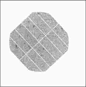
Now to continue, you need to measure the amount of noise in the image, you will then be able to determine a suitable threshold to use, so that most of the noise peaks lie below your threshold. Open up the inverted image Lockman_05_2inv.tif and draw a rectangular box in a particularly empty region of the image using the rectangular tool in the tool bar. Be careful when drawing this box as the useful part of the image does not extend to the edges of the window. (see the image below). Once the box is drawn, open the Analyze menu and click on Measure. In the info box some numbers will apear. The ones that are of interest are the average value and its standard deviation. Depending on exactly which region you have chosen, the mean should be around 1.6 and the standard deviation about 1.4 to 1.7. A good rule of thumb is that that few noise peaks should extend to a height as much as 5 times the standard deviation above the mean background level. We will now use this rule.

Firstly click on the image outside of the rectangular box you drew to select the whole image again. Now put the image back into threshold mode and set the threshold to 5 times the standard deviation above your mean background value, which should be about 9.  Once the threshold is set, open the Analyze menu and click on Set scale. Change the units to pixels, and then click ok. In the Analyze menu still, click on Options. In the options menu check the X-Y Center box, and ensure Area and Mean Density are also checked, and click ok.

     Now in the Analyze menu again, click on Analyze particles, and set the minimum particle size to 2 this time, and click ok. Now you can see that even with the minimum particle size set to 2, which is rather small  for a real source, there are only 44 detected peaks for a threshold of 9.

     Although setting a high threshold will avoid many of the noise peaks, it also means that we will miss any real weak sources in the field, so now we will try to do something about suppressing the noise.

Step 3 - Noise reduction

     The next stage of the process is to reduce the effect of noise and eliminate the background. To begin, open up the inverted image again, e.g Lockman_02_05inv.tif and find an area on the image which does not appear to contain much, i.e is a pale region. Then follow the steps as before to find the standard deviation and mean value in this region.

     The mean value corresponds to a background count and the standard deviation gives a representation of the amount of noise in the image. The value given for the mean background reading should be in the region 1.3 to 1.6 for the image Lockman_05_2. So now you should remove the background from the image by subtracting the mean value obtained from the values of all of the pixels. This is done by clicking on Process, scrolling down to Arithmetic, and then clicking subtract, then entering the value you obtained and clicking ok.

     With the background removed measure the small area again and check to see if it has fallen to zero, or a value close to zero. The value you get may not be zero because the program will only subtract integer values from the image , so if the mean is 1.17 , and you try and subtract this value, then in fact only 1 will be subtracted. Also do not worry if you don't select the exact area as before, you should still get a value close to zero.

     Having dealt with the issue of background, you can now deal with the noise. The method that will be used for reducing the amount of noise in the image is called smoothing. This is a process which blurs the image and the amount of smoothing can be varied. To smooth the image select the whole image again and then click on Process and then Convolve. Then select the Kernels folder in the Scion image directory and then select the file named smoothing1.txt. The image should now look slightly blurred.

     Now repeat the step used previously to find the background value and look at the standard deviation value. You should see that the value has reduced from what it was before smoothing the image. Now take a note of this value as it will be used in the next stage.

     You may be asking "how did we know that the amount of smoothing used was a reasonable amount to use?" It may seem that if smoothing reduces the amount of noise that doing more smoothing would provide more accurate results. Keeping the image you have just smoothed open, load in the original image again and try using the file smoothing2.txt on it instead, this kernel is larger than the first one and so produces more smoothing. This clearly shows that over smoothing doesn't help at all and just merges sources together if they are close together. Find the standard deviation in an empty region of this image and then save this over-smoothed image as lockman_05_2over.tif.

The key to choosing how much smoothing should be done is to note the size of the sources in the image. The kernel smoothing1.text has a width of 5 pixels, and this is about the size of a source in the image, and therefore it produces an appropriate amount of smoothing. The second kernel has a width of 15 pixels and so it over-smooths the image and reduces the number of sources that can be found.

    Step 4 - Re-doing the source find

     Using the image that has had its background removed and was smoothed using smoothing1.txt, i.e. lockman_05_2smoothed.tif, you need to redo the source find. Now it was said before that the standard deviation that was obtained after smoothing before would be important. This is where it is used. Now to find the sources again you need to set a threshold for the image. The new threshold that will be used is 5 times the standard deviation value previously obtained for the smoothed image (round up to the nearest integer) plus the mean background which is now zero. So if after background removal and smoothing your standard deviation was 0.7, then the threshold used will be 4.

     This time you should see that there are more sources found than before.

     Now do the same thing to the oversmoothed image using the Standard deviation value obtained from it. You can see that there are fewer sources found. This proves that over-smoothing is damaging to the results.

     In this exercise you have learned about the following:

• Preparing an image to be used for source finding
• Thresholding and using standard deviations to determine what value to use
• Noise and background 
• Smoothing and its effects on noise