


|
Exercise 3 - Hardness ratios |
|
What are Hardness ratios?
The range of X-ray energies which XMM can detect is very broad. Photons whose energy lies between 0.2 and 12.0 keV are used by the three cameras on the spacecraft to construct images, and as the energy as well as the position of each one is recorded, it is possible to make images with smaller energy ranges (or "bands"). Although most X-ray sources emit X-rays at a range of energies, different sources will have different emission profiles - for example, black holes and X-ray binaries typically emit a large fraction of their X-rays at high energies, whereas the hot gas seen in elliptical galaxies and starbursts usually has only a small high energy component. These differences are a consequence of the different physical processes which produce the X-rays. It is also important to note that the energy of the X-rays emitted is often determined by the temperature of the source. Heating metal will cause it to begin to glow, emitting photons in the optical range. As it gets hotter this glow will change from red, through orange, to white, as the peak energy of the photons becomes higher. Astronomical objects are often found to have temperatures of millions of Kelvin, so the peak energy of the photons they emit is in the X-ray regime. By measuring the energies of the photons, we can often determine the temperature of the source which emitted them.
In general terms, astronomers refer to an X-ray source as being "hard" if a large percentage of its X-ray emission is at higher energies, or "soft" if it mainly produces lower energy photons. The "hardness" of a source therefore gives a rough idea of what sort of X-ray emission we are looking at, and sometimes of the temperature of the source. A more accurate estimate can be obtained by calculating hardness ratios. If we observe an X-ray source and then construct images in different energy bands, we can count the number of photons we have detected in each band, and calculate the ratios between them. By using standard bands when looking at different sources, we can find out what ratios we would expect for each different type of object. Then, when we come to look at a new object, its hardness ratios will allow us to classify it quickly.
This exercise aims to show you the advantages of observing objects in different energy bands, and demonstrate how to calculate hardness ratios. Using the supernova remnant images previously downloaded from the image library, you will be shown how the structure of the object varies with energy.
Step 1 - Preparing the ImagesFirstly start up Scion Image and use the Open command in the File menu to open the first of the supernova remnant images, CasA_SNR_1.tif. As described in exercise 1, before we can use the image we need to carry out procedures to remove the background and reduce the level of noise in the image. First, select Invert from the Edit menu, to produce an image in black on a white background. The supernova remnant (SNR) should be visible as a roughly circular object at the centre of the image. Next, use the box or circle tool to select a featureless region near the SNR. Go to Analyze -> Options and make sure Area, Mean Density and Integrated Density are selected. If you then select Measure from the Analyze menu, you should see values for this region appear in the Info window. The mean value gives an estimate of the background level of the image. A value of between 2 and 5 is to be expected for this image. Click elsewhere on the image to de-select the region, and use Process -> Arithmetic -> Subtract and subtract this mean value from the whole image. This will remove background emission from the image. Then select Process -> Convolve and pick the file smoothing1.txt form the kernels directory. This should reduce the noise level in the image, and make the SNR look rather unfocused. If you now redraw your region on the image and remeasure the values in it, you should find a mean value of less than 1, indicating that your image has been cleaned of unwanted emission. You must now save this image preferably under a similar name, such as CasA_smooth_1.tif. Now repeat this cleaning operation for the other four supernova remnant images.
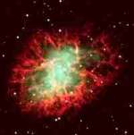
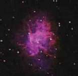
Morphology at different EnergiesThe five images you have cleaned are pictures of the Cassiopeia A supernova remnant. The images are taken in different energy bands, as shown in the table below. You may have noticed while preparing them that the images do not all look the same. At the basic level, supernova remnants are spherical shells of hot gas, expanding outward from the original site of the supernova explosion. However, in reality this shell is unlikely to be perfectly spherical. It is likely that as the gas moves outwards it will collide with cool gas in the region surrounding the star. These collisions can heat up both the cool gas and the hot gas from the supernova, causing them to emit X-rays and making that part of the SNR look brighter. The original supernova may also have been asymmetrical. We therefore expect the SNR to look clumpy, and not necessarily circular. We also expect it to look different at different energies, as different parts of the remnant undergo different interactions with the environment around them.
In the case of Cassiopeia A, we believe that there are several components to the emission. The coolest is made up mainly from gas that was in the outer layers of the star during the supernova explosion. Most photons from this component have energies of 0.3-1.0 keV, and the gas contains many ions of Silicon, Sulphur, Argon and Calcium. There is a hotter gaseous component, emitting photons of 2.0-6.0 keV, which contains more Iron and Nickel than the cooler component. This is likely to have come from the core of the star, and it is thought to have been blown out of the star not in a spherical shell, but as "bullets" of material in two jets along the polar axis. There is also a very high temperature (12.0-15.0 keV) component to the X-ray emission, which is thought to be caused by radiation from very high energy electrons accelerated by the magnetic forces produced during the supernova explosion.
| Image no. | 1 | 2 | 3 | 4 | 5 |
| Band (keV) | 0.2-0.5 | 0.5-2.0 | 2.0-4.5 | 4.5-7.5 | 7.5-12.0 |
In order to see more clearly the way in which the morphology of the SNR changes with energy band, we can combine the images to make a short animation. First, open all the images in order, so that you have five image windows on the screen. Then select Windows to Stack from the Stacks menu. This should collapse all the image windows into a single window with the title "Stack[1/5]". The five images are now combined on top of one another as a stack. You can cycle through the images either by using the Next Slice or Previous Slice commands in the Stacks menu, or by pressing Ctrl+, or Ctrl+.. By holding down these keys you can cycle quickly through all five images. You should be able to see that the soft (low energy) emission is most found on the upper left of the SNR, while upper right quadrant has more hard (high energy) emission.
Scion image is also able to cycle through the images automatically, to form a looped animation. Select Animate from the Stacks menu to see this. You may find that the initial speed of the animation is too fast or too slow. You can control the animation speed using the number keys, with 1 being slowest and 9 fastest. You can stop the animation by clicking on the image window. When you are happy with the speed, try to identify some areas of the SNR which appear brightest in the softer and harder bands. You can the use these to calculate harness ratios, as described below.
Calculating Hardness ratiosHardness ratios are calculated based on the number of detected photons in a region, in different bands. The first thing we need to do is define this region. You need to pick a section of the SNR which appears bright in some bands and faint in others. Next use the rectangle drawing tool to place a box around this region. As you want to use this region on several images, you need to save it, using the Save As... option on the File menu. In the Save As window which opens, change the file type to Outline[.ROI], and give your file a name, e.g. Region1.ROI. This file will contain the details of the box you have drawn, and you can now draw the box on any image simply by re-loading this file.
Having saved this box, you should now choose another region which appears brightest in a different band. Save this region under a separate file name, and repeat the process for any other regions you wish to look at. In this example, we have selected three regions, one covering the upper left quadrant of the SNR, one the lower left, and one the lower right quadrant. The values given below will refer to these three regions, but don't worry if your values are somewhat different - the size and position of the regions chosen can make quite a bit of difference.
To calculate simple hardness ratios, we need to count the number of photons in the regions selected in at least two bands. Images 2 and 4 are probably the best choices. Open the softer image (image 2 in this example) and load one of the region files by selecting Open from the File menu. If you then select Measure from the Analyze menu, you will see the values for this region appear in the Info window. The value we are interested in is The Integrated density. You will need to note down this number, and may find it useful to construct a table such as the one below. Load each region and measure the number of photons in it, noting each value. Then repeat the process for the Hard band image (image 4).
| Region no | Position | Soft Band | Hard Band |
| 1 | Lower right | 3724 | 34126 |
| 2 | Upper left | 43314 | 11365 |
| 3 | Lower left | 38184 | 22889 |
The hardness ratio is defined as
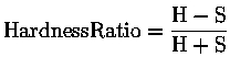 |
where H and S represent the number of photons counted in the hard and soft bands. Taking the measured numbers for your regions, you can calculate the ratios for your regions. The table below shows the hardness ratios calculated for our example regions. Positive values indicate that a source is hard, negative values that it is soft. For our regions it is clear that region 1 contains very hard emission, while region 2 is considerably softer. Region 3 is between these two, but is still mainly comprised of soft emission. This suggests that region 1 contains more of the hot gaseous component of the SNR, and is Iron-rich. Regions 2 & 3 are probably mainly comprised of the cooler gas from the outer layers of the progenitor star.
| Region no | Hardness Ratio |
| 1 | +0.803 |
| 2 | -0.584 |
| 3 | -0.250 |
The example given here is quite a simple one. In practice hardness ratios are most commonly used to look at relatively point-like sources from which we only detect a few photons. One thing which you can try is to use larger and smaller regions to compare the hardness ratios of small knots of emission in the SNR with those of more extended regions. Are the clumps harder or softer, or does this vary depending on where they are? We might expect some of the small knots visible in images 4 and 5 to have been produced from the "bullets" of hot material thrown out from the core of the star. Can you find any examples which might support this hypothesis?
SUMMARY
In this exercise you have learned about the following:
- The use of multiple energy bands in X-ray astronomy
- Calculating and comparing hardness ratios
- Variations in the morphology of objects at different energies
|
|